PCR Primer and Probe Design: A Comprehensive Guide from Principles to Validation for Researchers
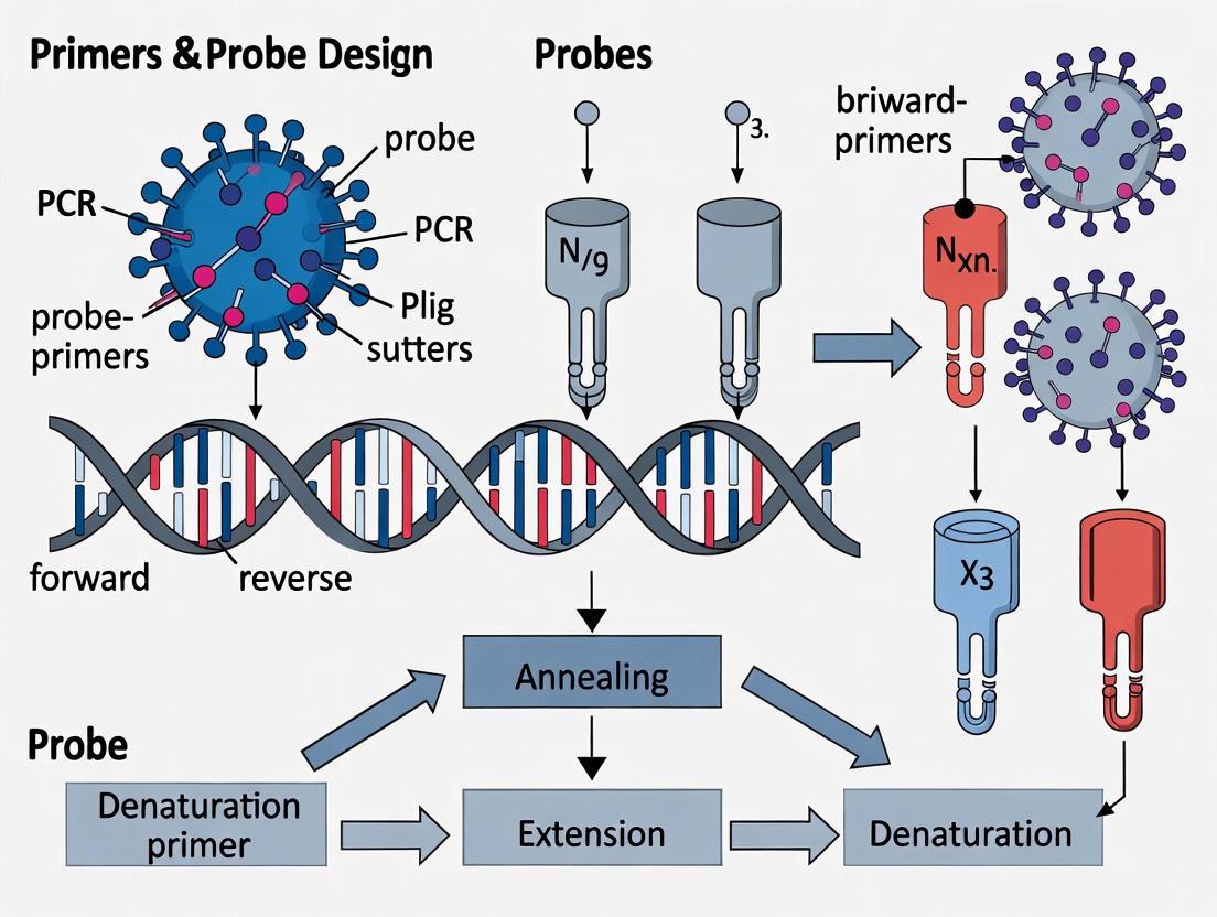
This article provides a complete framework for designing, optimizing, and validating primers and probes for PCR, qPCR, and dPCR assays.
PCR Primer and Probe Design: A Comprehensive Guide from Principles to Validation for Researchers
Abstract
This article provides a complete framework for designing, optimizing, and validating primers and probes for PCR, qPCR, and dPCR assays. Tailored for researchers and drug development professionals, it covers foundational principles, advanced methodologies for specific applications like bisulfite sequencing and multiplexing, systematic troubleshooting of common issues, and rigorous validation techniques adhering to MIQE guidelines. The guide synthesizes current best practices and tools to ensure the development of robust, specific, and efficient molecular assays for reliable research and diagnostic outcomes.
Core Principles of PCR Primer and Probe Design: Building a Solid Foundation
Within the broader context of primers and probe design for PCR assays, the meticulous optimization of physical and chemical parameters is fundamental to successful assay development. Polymerase Chain Reaction (PCR) serves as a cornerstone technology in molecular biology, diagnostics, and drug development, with its efficacy critically dependent on the effective design of oligonucleotide primers. This application note details the three pivotal parameters—primer length, melting temperature (Tm), and GC content—providing researchers with structured data, detailed protocols, and practical tools to ensure robust and specific amplification in their experiments.
Parameter Specifications and Quantitative Summaries
Primer Length
Primer length directly influences both the specificity and the efficiency of primer binding. Excessively short primers can lead to nonspecific amplification, whereas overly long primers may reduce the hybridization rate and are not typically necessary for most applications [1] [2].
Table 1: Specifications for Primer Length
| Parameter | Specification | Rationale |
|---|---|---|
| Optimal Range | 18 - 30 nucleotides [1] | Balances binding efficiency with sufficient specificity for accurate targeting. |
| Typical Use | 20 - 24 nucleotides [2] | A standard length suitable for a wide array of PCR applications. |
| Impact of Short Primers | < 18 nucleotides | High risk of nonspecific amplification and inaccurate products [2]. |
| Impact of Long Primers | > 30 nucleotides | Can result in a slower hybridization rate [2]. |
Melting Temperature (Tm)
The melting temperature (Tm) is defined as the temperature at which half of the DNA duplex dissociates into single strands. It is crucial that the forward and reverse primers in a pair have closely matched Tms to ensure both bind to the template simultaneously during the annealing step [1] [3].
Table 2: Specifications for Melting Temperature (Tm)
| Parameter | Specification | Rationale |
|---|---|---|
| Optimal Tm Range | 65°C - 75°C [1] | Provides a sufficiently high temperature to promote specific hybridization. |
| Alternative Tm Range | 50°C - 60°C [2] | A common range for many standard PCR protocols. |
| Primer Pair Tm Match | Within 5°C of each other [1] [2] | Ensures both primers anneal with similar efficiency. |
| Key Influencing Factors | Primer length, nucleotide composition (GC vs. AT), and buffer conditions [1] [4] | G and C bases, which form three hydrogen bonds, result in a higher Tm than A and T bases [1]. |
GC Content
GC content refers to the percentage of nitrogenous bases in the primer that are either Guanine (G) or Cytosine (C). Since GC base pairs are stabilized by three hydrogen bonds (compared to two for AT pairs), the GC content directly affects the primer's stability and binding strength [5].
Table 3: Specifications for GC Content
| Parameter | Specification | Rationale |
|---|---|---|
| Optimal Range | 40% - 60% [1] [2] | Balances primer stability and specificity. |
| GC Clamp | 1-2 G or C bases at the 3' end [2] | Promotes stronger binding at the 3' end, which is critical for enzyme elongation. |
| Distribution | Balanced distribution of GC-rich and AT-rich domains [1] | Avoids stretches of a single base type. |
| High GC Content | >60% | May necessitate higher annealing temperatures and can promote non-specific binding or stable secondary structures [5] [3]. |
Experimental Protocols for Parameter Determination
Protocol for Calculating GC Content
The GC content is a fundamental property derived directly from the primer sequence.
Procedure:
- Sequence Input: Obtain the nucleotide sequence of the primer (5' to 3').
- Base Count: Count the total number of Guanine (G) and Cytosine (C) bases within the sequence.
- Calculation: Apply the following formula:
% GC Content = (Number of G + Number of C) / Total Number of Bases in Primer) * 100 - Verification: Utilize online tools, such as the VectorBuilder GC Content Calculator, to verify manual calculations and visualize base distribution [5].
Protocol for Calculating Melting Temperature (Tm)
The Tm can be calculated using different formulas depending on the primer length. It is important to note that these are estimates, and empirical optimization may be required.
Procedure:
- Determine Primer Length (N):
N= Total number of nucleotides in the primer.
- Select the Appropriate Formula:
- For primers shorter than 14 nucleotides: Use the Wallace rule formula.
Tm = (wA + xT) * 2 + (yG + zC) * 4where w, x, y, z are the counts of A, T, G, and C bases, respectively [4]. - For primers 14 nucleotides or longer: Use the more sophisticated formula that accounts for salt concentration.
Tm = 64.9 + 41 * (yG + zC - 16.4) / (wA + xT + yG + zC)This formula assumes standard conditions of 50 nM primer and 50 mM Na+ [4].
- For primers shorter than 14 nucleotides: Use the Wallace rule formula.
- Use a Specialized Tm Calculator: For greater accuracy that incorporates specific reaction conditions (e.g., polymerase buffer composition, divalent cation concentration), use an online calculator such as the Thermo Fisher Tm Calculator [6] or the IDT OligoAnalyzer [7]. These tools employ advanced thermodynamic models for precise predictions.
Interrelationship of Primer Design Parameters
The core parameters of primer design do not function in isolation; they are intrinsically linked and must be balanced to achieve optimal PCR performance. The following diagram illustrates the logical relationships and primary design goals for these parameters.
The Scientist's Toolkit: Research Reagent Solutions
Table 4: Essential Tools and Reagents for Primer Design and Analysis
| Tool / Reagent | Function / Application | Example Providers / Resources |
|---|---|---|
| Online Tm Calculators | Calculates primer melting temperature based on sequence and buffer conditions. Critical for determining annealing temperatures. | Thermo Fisher [6], NEB [8], IDT OligoAnalyzer [7] |
| GC Content Calculator | Determines the guanine-cytosine percentage of a primer or sequence. | VectorBuilder [5] |
| Primer Specificity Tool | Checks primer pairs for specificity against a database to minimize off-target amplification. | NCBI Primer-BLAST [9] |
| Secondary Structure Analyzer | Predicts potential hairpins or self-dimers within a primer sequence. | IDT OligoAnalyzer (Hairpin, Self-Dimer functions) [7] |
| High-Fidelity DNA Polymerase | Enzymes with proofreading activity for high-accuracy amplification of complex or GC-rich templates. | New England Biolabs (NEB), Thermo Fisher Scientific |
| HPLC-Purified Primers | High-purity oligonucleotides via High-Performance Liquid Chromatography; recommended for cloning and critical applications to reduce synthesis failure products [1] [3]. | Various oligo synthesis vendors |
Within the broader context of designing robust primers and probes for PCR assays, ensuring specificity is a cornerstone of reliable data in molecular biology research and drug development. A significant challenge to this specificity is the formation of primer secondary structures, such as hairpins, and inter-primer interactions, notably primer-dimers. These aberrant structures arise from complementary base pairing within a single primer or between two primers, effectively competing with the target DNA template during the annealing phase of the PCR [10] [11]. The consequences include reduced amplification efficiency, lower yield of the desired product, inaccurate quantification in quantitative PCR (qPCR), and potential false positives [12] [13]. This application note details the principles and protocols for designing primers that avoid these pitfalls and for experimentally troubleshooting their formation, providing essential knowledge for researchers and scientists focused on assay development.
Principles of Specific Primer Design
The foundation for avoiding secondary structures and dimerization lies in meticulous in silico primer design. Adherence to established design parameters drastically reduces the potential for non-specific interactions.
Key Design Parameters
The following parameters should be evaluated for every primer set before proceeding to experimental validation [1] [14] [15].
- Primer Length: Optimal primer length is generally 18–30 nucleotides [1] [14]. Shorter primers bind more efficiently but may lack specificity, while longer primers can hybridize too slowly.
- Melting Temperature (Tm): The Tm for both forward and reverse primers should be between 60°C and 75°C, and within 5°C of each other to ensure simultaneous and specific binding during the annealing step [1] [15].
- GC Content: Aim for a GC content of 40–60% [1] [11]. This provides sufficient sequence complexity and binding strength without promoting non-specific annealing. A maximum of 3 G or C bases in the last 5 nucleotides at the 3' end (a "GC clamp") is beneficial for specific initiation but avoid more than 3 to prevent mispriming [1] [11].
- Self-Complementarity: Primers must be screened for regions that are complementary to themselves (which can form hairpins) or to the other primer in the pair (which can form primer-dimers). The key is to minimize complementary regions, especially at the 3' end where the polymerase extends [1].
- Runs and Repeats: Avoid runs of four or more identical bases (e.g., AAAA) or dinucleotide repeats (e.g., ATATAT), as these can cause mispriming [1] [14].
Quantitative Design Thresholds
The table below summarizes the critical thresholds for key parameters to minimize secondary structures and dimer formation.
Table 1: Key Primer Design Parameters and Their Optimal Ranges
| Parameter | Optimal Range | Rationale & Avoidance |
|---|---|---|
| Length | 18–30 nucleotides [1] [14] | Balances efficient binding and sufficient specificity. |
| Tm | 60–75°C; primers within 5°C of each other [1] [15] | Ensures simultaneous and specific annealing of both primers. |
| GC Content | 40–60% [1] [11] | Provides stable binding without excessive non-specific interactions. |
| GC Clamp | 2-3 G/C bases in the last 5 nucleotides at 3' end [1] [11] [14] | Promotes specific binding at the site of polymerase extension. |
| Self-Dimer/ Hairpin ΔG | > -9.0 kcal/mol [15] [16] | A less negative (more positive) ΔG value indicates a stable secondary structure is unlikely to form. |
| 3' Complementarity | Avoid complementarity of ≥ 3 bases between primers [1] | Prevents polymerase extension from a primer-dimer complex. |
In Silico Evaluation Workflow
A systematic workflow should be employed to design and evaluate primers prior to synthesis. The following diagram outlines the critical steps for in silico analysis.
Diagram 1: In silico primer design and evaluation workflow. Primers must pass checks for sequence composition, secondary structure potential, and specificity before being ordered.
Experimental Protocols for Detection and Optimization
Even with careful in silico design, experimental validation is crucial. This section provides protocols for detecting and troubleshooting secondary structures and primer-dimers.
Protocol: Identifying Primer-Dimers by Gel Electrophoresis
Primer-dimers can be visually identified and distinguished from the desired amplicon using agarose gel electrophoresis [10].
Key Characteristics of Primer-Dimers:
- Short Length: Typically appear below 100 bp due to the short length of the primers themselves.
- Smeary Appearance: Often manifest as a fuzzy, diffuse band rather than a sharp, well-defined one, indicating a heterogeneous mixture of nonspecific products.
Procedure:
- Prepare a standard PCR reaction mix including your primers, template, polymerase, dNTPs, and buffer.
- Critical Control: Include a No-Template Control (NTC). This reaction contains all components except the DNA template. Amplification in the NTC is almost certainly due to primer-dimer formation [10].
- Run the PCR using your initial thermal cycling parameters.
- Load the PCR products and an appropriate DNA ladder onto an agarose gel for electrophoresis.
- Run the gel longer than usual if necessary, to ensure small primer-dimer fragments are well-separated from the dye front and any specific, larger amplicons [10].
Interpretation: The desired amplicon should be a single, sharp band at the expected size, present only in the template-positive reactions. Primer-dimers will appear as a smeary band near the bottom of the gel in both test reactions and, tellingly, in the NTC.
Protocol: Using Free-Solution Conjugate Electrophoresis (FSCE) for Quantitative Dimer Analysis
For a more precise, quantitative analysis of dimerization, FSCE provides high-resolution data on primer-dimer stability under different conditions [17].
Principle: One primer is conjugated to a neutral "drag-tag" (e.g., a synthetic polyamide), which alters its electrophoretic mobility. When conjugated and non-conjugated primers form a dimer, the resulting duplex has a distinct mobility shift that can be separated and quantified using capillary electrophoresis without a sieving matrix [17].
Procedure:
- Sample Preparation: Design primers with partial complementarity. Conjugate one primer (e.g., a 30-mer) at its 5' end with a drag-tag via a thiol-maleimide linkage [17].
- Annealing: Mix drag-tagged and non-drag-tagged primers. Heat-denature at 95°C for 5 minutes, then anneal at a defined temperature (e.g., 62°C for 10 minutes) before cooling [17].
- Electrophoresis: Load samples onto a capillary electrophoresis system using a suitable buffer (e.g., 1x TTE). Perform separations at a range of temperatures (18°C, 25°C, 40°C, 55°C, 62°C) to assess the temperature dependence of dimer formation [17].
- Analysis: Quantify the peak areas corresponding to free primers and primer-dimer complexes. The proportion of dimer formed provides a quantitative measure of dimerization risk.
Key Experimental Findings: FSCE studies have empirically demonstrated that stable primer-dimer formation requires more than 15 consecutive base pairs. Non-consecutive base pairing, even with up to 20 out of 30 possible bonds, does not typically form stable dimers. Dimerization is also inversely correlated with temperature [17].
Protocol: Optimization Strategies to Suppress Dimer Formation
If primer-dimers are detected, the following experimental optimization strategies can be employed.
- Adjust Primer Concentration: Lowering the primer concentration reduces the probability of primers encountering each other instead of the template. A typical starting range is 0.1–0.5 µM [10].
- Increase Annealing Temperature: Systematically increase the annealing temperature in 1–2°C increments. A higher temperature favors specific (perfect-match) binding and disrupts the weaker bonds in primer-dimers [10] [13].
- Utilize Hot-Start Polymerases: These enzymes remain inactive until a high-temperature activation step (e.g., 95°C), preventing non-specific extension and dimer formation during reaction setup and the initial thermal ramp [10] [13].
- Employ Touchdown PCR: This technique starts with an annealing temperature above the calculated Tm and gradually decreases it in subsequent cycles. This enriches for specific amplicons in the early cycles, which then out-compete non-specific products in later cycles.
The logical relationship between a detected problem and the available optimization strategies is outlined below.
Diagram 2: Experimental optimization strategies for troubleshooting primer-dimer formation. Strategies can be combined for greater effect.
The Scientist's Toolkit: Essential Reagents and Materials
The following table lists key reagents and materials required for the experiments and evaluations described in this application note.
Table 2: Essential Research Reagents and Materials for Primer Specificity Work
| Item | Function/Application |
|---|---|
| Hot-Start DNA Polymerase | Enzyme that remains inactive at room temperature, preventing non-specific extension and primer-dimer formation during PCR setup [10]. |
| Agarose Gel Electrophoresis System | Standard method for visualizing PCR products and identifying primer-dimers by size and band morphology [10]. |
| Capillary Electrophoresis System | Used for high-resolution, quantitative methods like FSCE to analyze dimer formation and purity of oligonucleotides [17]. |
| Synthetic Drag-Tags (e.g., NMEGs) | Neutral, water-soluble polymers conjugated to primers in FSCE to alter their hydrodynamic drag and enable mobility shift assays [17]. |
| Fluorophore-Labeled Nucleotides (FAM, ROX) | Used for fluorescent detection of DNA in capillary electrophoresis and real-time PCR applications [17]. |
| Primer Design Software (e.g., IDT OligoAnalyzer) | Online tools for calculating Tm, GC%, and analyzing self-dimers, hairpins, and cross-dimers via ΔG values [15] [16]. |
| Nuclease-Free Water | Essential for preparing all reaction mixes to prevent RNase and DNase contamination that could degrade primers and templates. |
The integrity of PCR-based data in research and diagnostic assays is fundamentally dependent on primer specificity. A rigorous, two-pronged approach combining stringent in silico design with empirical experimental validation is paramount for success. By adhering to the design principles outlined here—paying close attention to Tm, GC content, and especially complementarity—researchers can preemptively avoid the most common causes of secondary structure and dimer formation. When dimers persist, the provided experimental protocols offer a clear path for detection, from simple gel-based identification to sophisticated quantitative analysis, and for effective optimization through adjustments to reaction components and thermal cycling conditions. Integrating these strategies ensures the development of robust, specific, and efficient PCR assays, thereby solidifying the reliability of results in drug development and scientific discovery.
Melting Temperature (Tm) Calculations and the Importance of Primer Pair Matching
In polymerase chain reaction (PCR) assays, the melting temperature (Tm) is a fundamental thermodynamic property defined as the temperature at which 50% of DNA duplexes dissociate into single strands [18]. Accurate prediction and matching of primer Tm values is arguably the most critical parameter for successful experimental outcomes, influencing specificity, amplification efficiency, and yield across diverse PCR applications including quantitative PCR, multiplex PCR, and high-throughput genomic analyses [18] [19]. Proper primer pair design, grounded in robust Tm calculation methods, ensures efficient annealing while minimizing non-specific amplification and primer-dimer formation, thereby supporting the integrity of research in drug development and molecular diagnostics [20] [21]. This guide details the principles, calculation methods, and practical protocols for Tm determination and primer matching to support robust assay development.
Theoretical Foundations of Melting Temperature
DNA Melting Dynamics and Thermodynamic Principles
The DNA melting process involves the transition from a double-stranded helix to single-stranded random coils as temperature increases. At the Tm, an equilibrium exists where half of the duplex molecules remain hybridized and half are dissociated [18]. This transition is governed by the thermodynamics of base pairing, where GC base pairs (with three hydrogen bonds) contribute more significantly to duplex stability than AT base pairs (with two hydrogen bonds) [18].
The stability of DNA duplexes depends on several sequence and environmental factors. Sequence length directly influences Tm, with longer oligonucleotides forming more stable duplexes. The GC content significantly affects stability due to the stronger bonding in GC pairs. Additionally, nearest-neighbor interactions demonstrate that base pair stability is context-dependent, influenced by adjacent nucleotides [18]. Solution conditions such as salt concentration (Na⁺, K⁺, Mg²⁺) stabilize duplexes by shielding the negative charge of the phosphate backbone, while additives like DMSO and formamide disrupt hydrogen bonding, thereby reducing observed Tm values [18].
Evolution of Tm Calculation Methods
The accuracy of Tm prediction has evolved substantially from simple empirical formulas to sophisticated thermodynamic models [18]. The historical GC% method (Tm = 4°C × GC% + 2°C × AT%) provided rough estimates but incurred significant errors (5-10°C) due to its neglect of sequence context and terminal effects [18]. Modern approaches utilize the SantaLucia nearest-neighbor method, which accounts for all ten possible dinucleotide pairings with experimentally determined thermodynamic parameters (ΔH and ΔS), delivering precision within 1-2°C of experimental values [18]. This method calculates Tm using the formula:
Tm = ΔH / (ΔS + R × ln(C/4)) - 273.15
Where ΔH is enthalpy, ΔS is entropy, R is the gas constant, and C is the oligonucleotide concentration [18].
Table 1: Comparison of Tm Calculation Methods
| Method | Accuracy | Key Parameters Considered | Best Application |
|---|---|---|---|
| Simple GC% Formula | ±5-10°C error | GC content only | Rough estimations |
| Basic Nearest-Neighbor | ±3-5°C error | Sequence context | General laboratory use |
| SantaLucia Method | ±1-2°C error | Sequence context, terminal effects, salt corrections | PCR, qPCR, research applications |
Tm Calculation Methods and Protocols
Step-by-Step Protocol: Using a Modern Tm Calculator
This protocol utilizes the SantaLucia nearest-neighbor method for accurate Tm prediction, suitable for PCR primer design, qPCR optimization, and hybridization assay development [18].
Materials Required
- DNA or RNA sequence of the oligonucleotide
- Tm calculator (online or stand-alone software implementing SantaLucia method)
- Buffer composition data for your specific PCR system
Procedure
Sequence Input: Paste your oligonucleotide sequence (DNA: A, T, C, G; RNA: A, U, C, G) into the input field. The tool typically accepts sequences with or without spaces, numbers, or line breaks [18].
Sequence Type Selection: Designate whether the input sequence is DNA or RNA from the dropdown menu to ensure application of appropriate thermodynamic parameters [18].
Salt Concentration Adjustment: Set monovalent (Na⁺/K⁺) and divalent (Mg²⁺) cation concentrations according to your experimental buffer conditions [18].
- For standard PCR: 50 mM Na⁺, 1.5-2.5 mM Mg²⁺
- For high-fidelity PCR: 20-30 mM Na⁺, 1-2 mM Mg²⁺
- For qPCR: 50-100 mM Na⁺, 3-5 mM Mg²⁺
- Note: If your buffer contains both Na⁺ and K⁺, use the total monovalent cation concentration [18].
Oligonucleotide Concentration Specification: Set concentration appropriate for your application [18]:
- PCR primers: 0.1-0.5 µM (0.25 µM standard)
- qPCR primers: 0.1-0.3 µM
- Probes: 0.05-0.2 µM
Additive Adjustment (Optional): If using DMSO, input the percentage (typically 5-10% for GC-rich templates). DMSO reduces Tm by approximately 0.6-0.7°C per 1% concentration [18].
Calculation Initiation: Click "Calculate Tm" to generate results including Tm value, thermodynamic parameters (ΔH, ΔS), GC content percentage, and sequence length [18].
Experimental Validation of Calculated Tm
While computational predictions provide excellent guidance, empirical validation remains essential for critical applications. Several methods exist for experimental Tm determination:
UV Spectrophotometry with Temperature Ramp: Monitor absorbance at 260 nm while increasing temperature by 0.5-1°C per minute. The Tm corresponds to the midpoint of the hyperchromic shift [19].
SYBR Green I Fluorescence Melting Curves: After PCR amplification, slowly increase temperature while monitoring fluorescence decrease. Plot the negative derivative of fluorescence versus temperature (-dF/dT) to identify the Tm peak [21].
Calorimetric Methods: Isothermal titration calorimetry (ITC) or differential scanning calorimetry (DSC) provide direct thermodynamic parameter measurements but require specialized instrumentation [19].
Primer Pair Matching and PCR Optimization
The Critical Importance of Tm Matching
Successful PCR amplification requires forward and reverse primers with closely matched Tm values to hybridize simultaneously to the template during the annealing step. Significant Tm discrepancies (>5°C) between primer pairs result in inefficient amplification, where the higher-Tm primer may anneal preferentially while the lower-Tm primer exhibits reduced binding, diminishing product yield and specificity [18] [22].
Statistical analyses of PCR failure rates across 1,147 mammalian primer pairs revealed that the number of primer-template mismatches significantly impacts amplification success, with each mismatch decreasing success probability by 6-8% [22]. Furthermore, GC-content within the amplified region substantially influences outcomes, with regions exceeding 50% GC showing reduced amplification efficiency (56.9% success versus 74.2% for GC<50%) in cross-species applications [22].
Protocol for Primer Pair Evaluation and Selection
This protocol ensures selection of compatible primer pairs with matched Tm values for robust PCR amplification.
Materials Required
- Forward and reverse primer sequences
- Tm calculator
- Template sequence for specificity checking
- Primer analysis software (e.g., NCBI Primer-BLAST)
Procedure
Calculate Individual Primer Tm Values: Using the protocol in section 3.1, determine Tm for both forward and reverse primers under identical reaction conditions [18].
Assess Tm Compatibility: Select primer pairs with Tm values differing by no more than 5°C. The ideal range for both primers is 55-65°C, with 58-62°C being optimal for most applications [18] [23].
Determine Optimal Annealing Temperature: Calculate the experimental annealing temperature (Ta) as 3-5°C below the lower Tm of the two primers [18]. For touchdown PCR, begin 5-10°C above the expected Tm and decrease by 0.5-1°C per cycle until reaching the calculated Ta.
Verify Primer Specificity: Utilize NCBI Primer-BLAST to confirm primer pair specificity to the intended target sequence, checking for potential off-target binding [9].
Evaluate Secondary Structures: Analyze primers for potential hairpins, self-dimers, and cross-dimers using tools like OligoAnalyzer. Avoid primers with stable secondary structures (ΔG < -5 kcal/mol) [23].
Check 3'-End Stability: Ensure primers terminate with G or C bases (GC clamp) to enhance binding specificity at the critical 3' end where extension initiates [23].
Table 2: Troubleshooting Guide for Primer Tm Issues
| Problem | Potential Causes | Solutions |
|---|---|---|
| Tm too low (<50°C) | Insufficient length, low GC content | Increase primer length to 25-30 nt, add G or C bases while maintaining 40-60% GC content |
| Tm too high (>70°C) | Excessive length, high GC content | Shorten primer to 18-22 nt, reduce GC content, or incorporate DMSO (5-10%) in reaction |
| Large Tm difference between pairs | Mismatched length or composition | Redesign one primer to match the other's Tm, adjusting length and GC content systematically |
| Non-specific amplification | Multiple binding sites, low Ta | Increase annealing temperature, verify specificity with Primer-BLAST, optimize Mg²⁺ concentration |
| Poor amplification efficiency | Secondary structures, 3' mismatches | Screen for hairpins and dimers, ensure 3' end stability, verify template quality and concentration |
Advanced Applications and Considerations
Specialized PCR Applications
Cross-Species Primer Design
When designing primers for amplification across species boundaries, additional considerations apply. Analysis of 1147 mammalian primer pairs demonstrated that amplification success significantly depends on the relatedness of the target species to the index species used for primer design [22]. The number of mismatches between index species in the primer binding region critically impacts success rates, with each mismatch decreasing amplification probability by 6-8% [22]. For cross-species applications, prioritize conserved genomic regions and verify amplification empirically across the intended species range.
Quantitative PCR (qPCR) Assays
qPCR applications demand exceptional primer precision to ensure accurate quantification. The MIQE guidelines emphasize the necessity of reporting primer sequences and validation data for publication [24]. For probe-based qPCR systems, the Tm of hybridization probes should be 5-10°C higher than the primer Tm to ensure probe binding precedes primer extension [21]. Statistical design of experiments (DOE) approaches can optimize probe configurations, significantly enhancing assay efficiency by up to 10% while reducing required optimization reactions [21].
High-Throughput and Multiplex PCR
In multiplex reactions employing multiple primer pairs, stringent Tm matching becomes exponentially more critical. All primers should exhibit Tm values within a 2-3°C range to ensure balanced amplification of all targets [18]. Computational prediction of PCR success using recurrent neural networks has demonstrated 70% accuracy in forecasting amplification outcomes from primer and template sequences alone, offering promising approaches for large-scale assay design [20].
Several software platforms implement robust Tm calculation algorithms suitable for research applications:
- Primer3 Plus/Primer3: Implements SantaLucia thermodynamics with comprehensive design capabilities [19]
- NCBI Primer-BLAST: Integrates Tm calculation with specificity verification against genomic databases [9]
- OligoAnalyzer Tool: Provides Tm calculation with secondary structure prediction
- Commercial primer design tools: Offer proprietary algorithms optimized for specific applications
Comparative analysis of 22 Tm calculator tools revealed that Primer3 Plus and Primer-BLAST provide the most accurate predictions, with minimal deviation from experimentally determined Tm values [19].
Research Reagent Solutions
Table 3: Essential Reagents for Tm Determination and PCR Optimization
| Reagent/Category | Function/Description | Application Notes |
|---|---|---|
| Thermostable DNA Polymerases | Enzymatic DNA synthesis | Selection influences buffer composition and optimal Mg²⁺ concentration |
| PCR Buffers with Mg²⁺ | Maintain pH and provide essential cofactors | Mg²⁺ concentration typically 1.5-2.5 mM; significantly impacts Tm |
| dNTP Mix | Nucleotide substrates for amplification | Standard concentration 200-250 µM each dNTP |
| DMSO (Dimethyl Sulfoxide) | Additive reducing DNA stability | Reduces Tm by 0.6-0.7°C per 1%; helpful for GC-rich templates (>60% GC) |
| Salt Solutions (KCl, (NH₄)₂SO₄) | Modifies ionic strength | Higher salt increases Tm; standard PCR: 50 mM K⁺ |
| SYBR Green I Dye | Fluorescent dsDNA binding | For melt curve analysis and experimental Tm validation |
| Commercial Tm Prediction Software | Computational Tm calculation | Implement SantaLucia method; essential for robust primer design |
Diagram 1: Primer Design and Tm Optimization Workflow. This flowchart illustrates the systematic process for designing PCR primers with optimized melting temperatures, including critical validation steps.
Annealing Temperature (Ta) Optimization for Maximum Efficiency
Within the broader context of primer and probe design research, the optimization of the annealing temperature (Ta) stands as a critical determinant for the success of any polymerase chain reaction (PCR) assay. Achieving maximum efficiency requires a meticulous balance, as an improperly optimized Ta can lead to nonspecific amplification, reduced yield, or complete amplification failure [15] [25]. This protocol details a systematic, stepwise approach to Ta optimization, integrating foundational principles with advanced strategies to ensure the development of robust, sensitive, and specific PCR assays suitable for demanding applications in research and drug development.
Theoretical Foundations of Annealing Temperature
The annealing temperature is defined as the temperature at which primers bind, or anneal, to the complementary target sequence in the template DNA during the PCR cycle. This step is paramount for determining the specificity and efficiency of the entire amplification reaction [26].
Relationship Between Tm and Ta
The optimal Ta is intrinsically linked to the melting temperature (Tm) of the primers. The Tm is the temperature at which 50% of the primer-template duplexes are dissociated [15]. A fundamental rule of thumb is to set the Ta 3–5°C below the calculated Tm of the primer with the lowest melting temperature [26]. This ensures sufficient stability for the primer to bind while minimizing the likelihood of non-specific binding.
- Ta Too Low: If the Ta is set excessively low, primers may tolerate mismatches and bind to non-target sequences, leading to non-specific amplification and a fuzzy background on an agarose gel [15] [25].
- Ta Too High: If the Ta is set too high, approaching or exceeding the primer's Tm, the probability of primer binding is significantly reduced. This leads to a sharp decrease in reaction efficiency and poor product yield [15].
Calculating Melting Temperature (Tm)
Accurate Tm calculation is the cornerstone of Ta optimization. Several formulas are commonly used, with varying levels of sophistication. Table 1 summarizes the most widely applied methods.
Table 1: Common Methods for Calculating Primer Melting Temperature (Tm)
| Method | Formula | Key Considerations |
|---|---|---|
| Basic Rule of Thumb | ( Tm = 4(G + C) + 2(A + T) ) | Quick estimation; ignores salt and primer concentration [26]. |
| Salt-Adjusted Formula | ( Tm = 81.5 + 16.6(log_{10}[Na^+]) + 0.41(\%GC) - 675/\text{primer length} ) | More accurate as it accounts for monovalent cation concentration [26]. |
| Nearest Neighbor Method | Uses thermodynamic stability of every adjacent dinucleotide pair. | Most accurate method; employed by modern online design tools (e.g., OligoAnalyzer, Primer3) [15] [26]. |
It is crucial to use the same Tm calculation method that your primer design software employs. Furthermore, the presence of PCR additives like DMSO or formamide can lower the effective Tm, necessitating a corresponding adjustment of the Ta [26].
Stepwise Optimization Protocol
A systematic approach to Ta optimization saves time and reagents while ensuring assay robustness. The following protocol outlines a comprehensive workflow, visualized in Figure 1.
Figure 1: A systematic workflow for the stepwise optimization of annealing temperature (Ta).
Preliminary Calculations and Setup
- Tm Calculation: Use the Nearest Neighbor method within a reliable online tool (e.g., IDT OligoAnalyzer, Primer3Plus) to calculate the Tm for both the forward and reverse primer. Use your specific reaction buffer conditions (e.g., 50 mM K+, 3 mM Mg2+) for an accurate calculation [15] [27].
- Define Initial Ta and Range: The initial Ta should be set 3–5°C below the lowest Tm of the primer pair [26]. For a gradient PCR, define a range that typically spans from 8°C below to 2°C below the lowest Tm [26].
Empirical Testing via Gradient PCR
- Prepare Master Mix: Prepare a single, large-volume master mix containing all reaction components (buffer, dNTPs, MgCl2, DNA polymerase, primers, and template). Aliquot this master mix evenly across PCR tubes or a multi-well plate. This ensures that the only variable across reactions is the temperature.
- Run Gradient PCR:
- Use a thermal cycler with a verified temperature gradient capability across its block [26].
- Program the cycler with the standard steps: initial denaturation (94–98°C for 1–3 min), followed by 25–35 cycles of denaturation (94–98°C for 15–30 s), annealing (gradient range for 30–60 s), and extension (68–72°C for 1 min/kb).
- End with a final extension (72°C for 5–10 min) [26].
Analysis and Selection
- Gel Electrophoresis: Analyze the PCR products using agarose gel electrophoresis.
- The optimal Ta condition will typically show a single, sharp band of the expected size against a clear background with minimal to no primer-dimer formations [25].
- qPCR Efficiency Calculation (If Applicable): For quantitative PCR (qPCR), further validation is required.
- Using the selected Ta, run a qPCR reaction with a serial dilution (e.g., 1:10) of the template to generate a standard curve.
- Calculate the amplification efficiency (E) using the slope of the standard curve: ( E = (10^{-1/slope} - 1) \times 100\% ).
- Optimal efficiency falls within the range of 90–110% (with 100% being ideal), accompanied by a correlation coefficient (R²) of ≥ 0.99 [27]. This high efficiency is a prerequisite for accurate relative quantification using the 2−ΔΔCt method [27].
Fine-Tuning and Troubleshooting
- If non-specific bands are observed: Increase the Ta in increments of 1–2°C and re-run the reaction [26] [25].
- If yield is low or no product is formed: Decrease the Ta in increments of 2–3°C or verify the integrity and design of the primers and template [26].
Advanced Optimization Strategies
Design of Experiments (DOE) for Multiparameter Optimization
Annealing temperature does not function in isolation. Its interaction with other components, especially MgCl2 concentration and primer concentration, can be significant. A Design of Experiments (DOE) approach allows for the systematic evaluation of these multiple factors and their interactions simultaneously, reducing the total number of experiments required [21]. For instance, one study used DOE to optimize a probe-based qPCR assay, successfully identifying key factors and reducing the number of individual reactions from 320 to 180 [21].
The Role of MgCl2 in Ta Optimization
Magnesium ion (Mg2+) concentration is a critical cofactor for DNA polymerase and stabilizes the primer-template duplex. There is a logarithmic relationship between MgCl2 concentration and the melting temperature of DNA [28]. A meta-analysis found that for every 0.5 mM increment in MgCl2 within the 1.5–3.0 mM range, the DNA melting temperature increases, thereby influencing the optimal Ta [28]. Therefore, if Ta optimization alone fails, a complementary titration of MgCl2 concentration (typically from 1.5 mM to 5 mM) is recommended [25] [28].
Universal Annealing for High-Throughput Applications
Some specialized reaction buffers contain isostabilizing components that allow for a universal annealing temperature (e.g., 60°C) to be used with a wide range of primers with different Tms. This can circumvent the need for extensive Ta optimization in applications like high-throughput screening [26].
Experimental Validation and Case Studies
Case Study: Optimizing a TaqMan qPCR Assay for Pathogen Detection
A 2025 study on optimizing a TaqMan qPCR for diagnosing Entamoeba histolytica provides a robust example of rigorous optimization [29].
- Objective: To identify the most efficient and specific primer-probe set and establish a logical cut-off Ct value.
- Methodology: The researchers designed 20 different primer-probe sets. They evaluated amplification efficacy using droplet digital PCR (ddPCR) by measuring absolute positive droplet counts and mean fluorescence intensity across different PCR cycles and annealing temperatures (59°C, 60°C, 61°C, and 62°C) [29].
- Key Finding: Of the initial five sets that showed high efficiency, only two maintained this efficiency at a higher annealing temperature of 62°C [29]. This highlights how empirical testing at different Ta values is critical for selecting the most robust assay, which may perform better under stricter thermal conditions.
Case Study: HRM Analysis for Malaria Speciation
Another 2025 study optimized a real-time PCR platform coupled with High-Resolution Melting (HRM) analysis for differentiating Plasmodium species [30].
- Protocol: The PCR was performed with an annealing temperature of 60°C.
- Outcome: The HRM method, building upon this optimized PCR, achieved a significant Tm difference of 2.73°C between P. falciparum and P. vivax, allowing for clear species differentiation. The results showed complete agreement with sequencing, validating the optimized protocol's accuracy [30].
The Scientist's Toolkit: Research Reagent Solutions
Table 2: Essential Reagents for Annealing Temperature Optimization
| Reagent / Tool | Function in Ta Optimization | Example & Notes |
|---|---|---|
| High-Fidelity DNA Polymerase | Provides robust activity and reduces mispriming at suboptimal Ta. | Enzymes from Archaea (e.g., Pfu) offer high thermostability for challenging conditions [26]. |
| Specialized PCR Buffers | Provides optimal pH and salt conditions; some enable universal annealing. | Buffers with isostabilizing components allow for a universal Ta (e.g., 60°C) [26]. |
| MgCl₂ Solution | Critical cofactor; concentration directly influences Tm and primer binding. | Requires titration (0.5-5.0 mM) in conjunction with Ta optimization [25] [28]. |
| PCR Enhancers | Can alter Tm and facilitate amplification of difficult templates (e.g., GC-rich). | DMSO, betaine, glycerol. Note: These typically lower the effective Ta [26]. |
| Gradient Thermal Cycler | Allows empirical testing of a temperature range in a single run. | Essential for efficient optimization. "Better-than-gradient" blocks provide precise well-level control [26]. |
| Online Tm Calculator | Calculates theoretical Tm using the Nearest Neighbor method. | IDT OligoAnalyzer Tool; use specific reaction conditions for accuracy [15]. |
| qPCR Standard Curve Materials | Validates amplification efficiency of the selected Ta. | Serial dilutions of a known template concentration are required [27]. |
The optimization of annealing temperature is a non-negotiable step in the development of a reliable PCR assay. By moving beyond simple calculations and adopting a systematic, empirical approach—starting with a temperature gradient and validating with efficiency calculations—researchers can achieve maximum amplification efficiency and specificity. Furthermore, considering the interplay of Ta with other reaction components, such as Mg2+ concentration, and leveraging advanced strategies like DOE, ensures the development of robust assays capable of meeting the stringent demands of modern scientific research and drug development.
The design of amplicons—the specific DNA sequences amplified by polymerase chain reaction (PCR)—is a foundational step in developing robust molecular assays. Among design parameters, amplicon length is a critical determinant of success, directly influencing amplification efficiency, specificity, and sensitivity. This parameter becomes especially crucial when working with fragmented DNA, a common characteristic of samples derived from formalin-fixed paraffin-embedded (FFPE) tissues, ancient DNA, and clinically relevant sources like cell-free DNA (cfDNA) from liquid biopsies [31]. In such contexts, the natural fragmentation of the DNA template imposes strict limitations on the maximum achievable amplicon size.
The relationship between amplicon length and template quality is not merely a technical consideration but a central principle in assay design. For instance, plasma cfDNA fragments exhibit a characteristic peak at approximately 167 base pairs (bp), reflecting nucleosomal protection [31]. Circulating tumor DNA (ctDNA) is often even shorter, presenting an opportunity for selective enrichment by designing shorter amplicons [31]. Failure to align amplicon length with the integrity of the source DNA can lead to drastic reductions in sensitivity or complete amplification failure. This application note details the strategic considerations and practical protocols for designing amplicons that are optimized for length, with a specific focus on challenging, fragmented DNA samples.
Core Principles of Amplicon Length Selection
General Guidelines for Different PCR Applications
The optimal amplicon length varies significantly depending on the specific PCR application and the quality of the starting template. The table below summarizes standard amplicon length recommendations for various common techniques.
Table 1: Recommended Amplicon Lengths for Various PCR Applications
| PCR Application | Recommended Amplicon Length | Key Considerations and Rationale |
|---|---|---|
| Standard PCR | 200 – 1000 bp [32] | Balances amplification efficiency with product specificity. Longer products may require increased extension times. |
| Quantitative PCR (qPCR) | 75 – 150 bp [32] | Shorter lengths promote high amplification efficiency and robust kinetics essential for accurate quantification. |
| Assays on Fragmented DNA (e.g., cfDNA, FFPE) | 70 – 140 bp [33] | Maximizes the probability of amplifying an intact target sequence from a fragmented DNA population. |
| Bisulfite PCR | 70 – 300 bp [33] | Bisulfite conversion is a harsh process that fragments and damages DNA, making shorter amplicons more reliable. |
| Long-Range PCR | > 3-4 kb [34] | Requires specialized polymerases and optimized cycling conditions to overcome challenges like depurination. |
The Critical Impact of Fragmented DNA
Fragmented DNA necessitates a paradigm shift in amplicon design. In standard PCR with high-quality genomic DNA, longer amplicons are often feasible. However, when the DNA template is degraded, the effective template length is determined by the size of the fragments, not the original genome.
- Liquid Biopsies and cfDNA: In non-invasive diagnostics using plasma cfDNA, the average fragment size is ~167 bp. Circulating tumor DNA (ctDNA) has been reported to be even shorter than cfDNA from healthy cells [31]. Designing amplicons that are shorter than the average fragment length is therefore essential to ensure a high probability that a given molecule is intact and can be amplified. For qPCR assays on such samples, amplicons of 70-140 bp are generally ideal [33].
- Bisulfite-Converted DNA: The chemical process of bisulfite conversion, used for methylation analysis, causes significant DNA fragmentation and damage. Consequently, PCR from bisulfite-converted DNA is more successful with shorter amplicons, typically kept between 70-300 bp, and often requires an increased number of PCR cycles (35-40) to compensate for the damaged template [33].
- Fundamental Design Rule: The guiding principle is to keep the amplicon shorter than the average DNA fragment size in the sample. This increases the likelihood that the entire region between the two primer binding sites is intact, allowing for successful amplification.
Experimental Protocols for Fragmented DNA Targets
Protocol 1: qPCR Assay Design for Cell-Free DNA
This protocol is optimized for generating short amplicons from cfDNA, such as from blood plasma, for sensitive detection in liquid biopsy applications [31] [33].
Workflow Overview:
Step-by-Step Procedure:
Template Assessment:
- Quantify and qualify the cfDNA using a high-sensitivity instrument (e.g., Bioanalyzer, TapeStation). Confirm the peak fragment size distribution is around 150-200 bp.
- Critical Step: Use this size profile to define the maximum allowable amplicon length.
Primer and Probe Design:
- Amplicon Length: Design the amplicon to be between 70 and 140 bp [33]. This ensures the amplicon is shorter than the majority of cfDNA fragments.
- Primer Length: Keep primers between 18-22 base pairs.
- Melting Temperature (Tm): Maintain the Tm of each primer between 55–70°C, with forward and reverse primers within 2°C of each other [33].
- GC Content: Design primers with a GC content of 40–60% without long stretches (>4) of the same nucleotide.
- Probe Design (for TaqMan): If using a hydrolysis probe, its Tm should be 4–8°C higher than the primers, and its length should be 20-25 bp [33].
In Silico Validation:
- Check primer sequences for self-complementarity, hairpins, and primer-dimer formation using tools like Primer3.
- Verify primer specificity by performing a BLAST search against the host genome (e.g., hg38 for human) to ensure binding is unique to the target [33].
Reaction Setup:
- Prepare a 20 µL reaction mix containing:
- 1X Hot-Start DNA Polymerase Master Mix (e.g., ZymoTaq)
- Forward and Reverse Primers: 0.3–1 µM each
- Probe (if applicable): 0.1–0.3 µM
- 5–20 ng of cfDNA template
- Use a high-sensitivity, hot-start polymerase to minimize nonspecific amplification and primer-dimer formation, which is critical for low-input samples.
- Prepare a 20 µL reaction mix containing:
Thermal Cycling:
- Use the following cycling conditions on a real-time PCR instrument:
- Initial Denaturation: 95°C for 2–5 minutes
- 40–45 Cycles of:
- Denaturation: 95°C for 10–15 seconds
- Annealing/Extension: 60°C for 30–60 seconds (acquire fluorescence here)
- The high cycle number compensates for the low abundance of the specific target in cfDNA.
- Use the following cycling conditions on a real-time PCR instrument:
Protocol 2: Long-Range Amplicon Sequencing for Structural Variation Analysis
This protocol is adapted for situations where longer amplicons are necessary, such as for sequencing to detect large deletions or structural variants, even from potentially compromised templates [35]. It emphasizes overcoming fragmentation challenges.
Workflow Overview:
Step-by-Step Procedure:
DNA Extraction and Long-Range PCR:
- Extract genomic DNA from your sample source (e.g., cell lines, primary cells).
- Perform long-range PCR to amplify a target region of 10–15 kb.
- Polymerase Selection: Use a high-fidelity, proofreading polymerase with minimal length bias, such as KOD (Multi & Epi) DNA polymerase, which has been shown to perform well for this application [35].
- Reaction Composition: Follow the manufacturer's recommendations for long-range PCR. This often includes balanced dNTP and Mg²⁺ concentrations, and potentially additives like DMSO for GC-rich regions.
- Cycling Conditions:
- Initial Denaturation: 95°C for 2 minutes.
- 30-35 Cycles of:
- Final Extension: 68°C for 5–10 minutes.
Amplicon Purification and Quality Control:
- Purify the PCR product using a magnetic bead-based clean-up system (e.g., AMPure XP beads) to remove primers, enzymes, and salts.
- Quantify the purified amplicon using a fluorometric method (e.g., Qubit dsDNA HS Assay) and check its integrity by agarose gel electrophoresis or a Fragment Analyzer.
Library Preparation and Sequencing:
- Fragment the purified long-range amplicon to ~300 bp using mechanical or enzymatic fragmentation.
- Prepare a sequencing library using a standard kit for Illumina platforms, including end-repair, dA-tailing, adapter ligation, and PCR enrichment steps.
- Sequence the library on an Illumina platform (e.g., MiSeq, NextSeq) to generate high-accuracy short reads.
Data Analysis for Large Variants:
- Analyze the sequencing data using a specialized tool like the ExCas-Analyzer, a k-mer alignment algorithm developed to simultaneously detect both small indels and large deletions (>100 bp) from long-range amplicon sequencing data [35].
- Standard genome aligners like BWA-mem may not be as sensitive for this specific application when dealing with large, complex indels near the CRISPR-cut site or target region.
The Scientist's Toolkit: Essential Reagents and Solutions
Successful amplicon generation, especially from fragmented DNA, relies on a carefully selected set of reagents and tools. The following table details key solutions for this field.
Table 2: Research Reagent Solutions for Amplicon-Based Studies
| Reagent / Tool | Function / Description | Application Notes |
|---|---|---|
| High-Sensitivity DNA Polymerase | Enzyme engineered for robust amplification from low-input and suboptimal templates. | Essential for qPCR of rare targets in cfDNA. Reduces primer-dimer formation [33]. |
| Proofreading DNA Polymerase | Enzyme with 3' to 5' exonuclease activity for high-fidelity synthesis of long amplicons. | Critical for long-range PCR to correct nucleotide misincorporations and ensure sequence accuracy [34]. |
| AMPure XP Beads | Magnetic beads for solid-phase reversible immobilization (SPRI) to purify and size-select DNA. | Used for post-PCR clean-up to remove primers and salts, and for library normalization in NGS workflows [36]. |
| ExCas-Analyzer Software | A dedicated k-mer alignment algorithm for analyzing long-range amplicon sequencing data. | Specifically detects both small indels and large deletions (>100 bp) with high accuracy and speed [35]. |
| Rapid Barcoding Kit (Oxford Nanopore) | Enables quick library preparation and multiplexing of amplicons for long-read sequencing. | Optimized for 500 bp to 5 kb amplicons; allows for sequencing of full-length fragments to check for mutations [36]. |
Strategic amplicon design, with length as a primary consideration, is a cornerstone of successful molecular assay development. The presented frameworks and protocols provide a roadmap for designing effective PCR-based assays across a spectrum of applications, from the highly sensitive detection of short cfDNA fragments in oncology to the sequencing of long amplicons for genetic variation studies. By aligning amplicon length with the biological and physical characteristics of the DNA template—especially its fragmentation profile—researchers and drug developers can significantly enhance the sensitivity, accuracy, and reliability of their genetic analyses. Adhering to these principles ensures that PCR assays are built on a robust foundation, ultimately leading to more dependable data and conclusions in both research and clinical settings.
Advanced Application-Specific Design: qPCR, RT-qPCR, Bisulfite, and Multiplexing
Within the broader context of PCR assay research, the design of TaqMan probes is a critical determinant for the success of quantitative real-time PCR (qPCR). These hydrolysis probes leverage the 5' nuclease activity of Taq polymerase to provide exceptional specificity and sensitivity for detecting and quantifying nucleic acid targets [37]. The reliability of this technique in diverse fields, from clinical diagnostics to fundamental gene expression analysis, is contingent upon a meticulously optimized primer-probe set [38]. This document outlines comprehensive application notes and protocols for designing TaqMan assays, with a focused examination of fluorophore and quencher selection, strategies to ensure target specificity, and detailed experimental methodologies.
Core Principles of TaqMan Probe Design
A TaqMan assay consists of a forward primer, a reverse primer, and a single-stranded DNA probe that is complementary to a specific sequence located between the two primer binding sites [39]. The probe is dual-labeled with a reporter fluorophore at its 5' end and a quencher molecule at its 3' end [40]. When the probe is intact, the proximity of the quencher to the reporter suppresses the reporter's fluorescence through a mechanism called Förster Resonance Energy Transfer (FRET) [37].
During the PCR amplification process, the TaqMan probe anneals to its specific target. As the Taq polymerase extends the primer, it encounters the bound probe and cleaves it via its 5' exonuclease activity. This cleavage separates the reporter dye from the quencher, leading to a permanent increase in fluorescence that is proportional to the amount of amplicon synthesized [37]. This process repeats every cycle, generating a fluorescent signal that directly correlates with the accumulation of the PCR product, without inhibiting the amplification itself [40] [37].
Visualizing the TaqMan Mechanism
The following diagram illustrates the step-by-step mechanism of the TaqMan probe hydrolysis during PCR amplification.
Fluorophore and Quencher Selection
The careful selection of the reporter fluorophore and quencher is paramount for achieving a high signal-to-noise ratio and for enabling multiplex assays where multiple targets are detected in a single reaction.
Reporter Fluorophores
Reporter dyes are characterized by their brightness, which is a product of their molar extinction coefficient and fluorescence quantum yield [41]. When selecting a fluorophore, researchers must balance optical performance with practical considerations like pH stability, photostability, and compatibility with the available real-time PCR instrument [41].
- Common Dyes: 6-FAM is the most frequently used reporter due to its high brightness [41]. Other common alternatives include VIC, TET, HEX, NED, ABY, and JUN [39] [42].
- Instrument Compatibility: Each qPCR instrument is equipped with a specific set of optical filters. It is essential to verify that the emission spectrum of the chosen reporter dye matches the instrument's detection capabilities. The table below summarizes compatible dyes for various common instruments [39] [42].
- Advanced Dyes: For challenging applications, dyes from the Alexa Fluor or ATTO series offer enhanced photostability and resistance to environmental factors like ozone, which can degrade traditional cyanine dyes (e.g., Cy5) [41].
Quenchers
The quencher's role is to absorb the energy from the reporter dye when they are in close proximity. Quenchers fall into two main categories: non-fluorescent quenchers (NFQs) and fluorescent quenchers.
- Non-Fluorescent Quenchers (NFQs): These are highly recommended because they do not emit background fluorescence, thereby improving the signal-to-noise ratio and making them ideal for multiplexing [39]. NFQs are often paired with specific modifications:
- MGB-NFQ: A Minor Groove Binder (MGB) moiety is conjugated to the NFQ. This stabilizes the probe's binding to the DNA, allowing for the use of shorter, more specific probes while maintaining a high melting temperature (Tm). This is especially beneficial for discriminating single-nucleotide polymorphisms (SNPs) [39].
- QSY Quencher: This is a non-fluorescent quencher without an MGB group. It is particularly suited for multiplexing three or more targets, as it offers high quenching efficiency without fluorescence [39].
- Fluorescent Quenchers: An example is TAMRA, which is a weakly fluorescent quencher. Its use consumes one of the instrument's detection channels in a multiplex setup and is generally less favored than NFQs [39].
Research Reagent Solutions
The following table details key reagents and their functions essential for TaqMan assay design and execution.
Table 1: Essential Research Reagents for TaqMan Assays
| Reagent Solution | Function & Description |
|---|---|
| Custom TaqMan Assays | Pre-mixed solutions containing forward primer, reverse primer, and a TaqMan probe with a specified fluorophore and quencher [39]. |
| Taq DNA Polymerase | Thermostable enzyme with both polymerase and 5' nuclease activity, essential for DNA amplification and probe hydrolysis [37]. |
| dNTPs | Deoxynucleotide triphosphates (dATP, dCTP, dGTP, dTTP); the building blocks for DNA synthesis. |
| qPCR Master Mix | Optimized buffer solution containing Taq polymerase, dNTPs, salts (MgCl₂, KCl), and a passive reference dye (e.g., ROX) [39]. |
| TE Buffer (pH 8.0) | Resuspension buffer (10 mM Tris-HCl, 1 mM EDTA) for lyophilized probes, ensuring stability and longevity [39] [42]. |
Instrument and Dye Compatibility
Selecting a fluorophore that is compatible with the detection system of your qPCR instrument is critical. The table below provides a reference for dye compatibility across common platforms.
Table 2: qPCR Instrument Dye Compatibility Guide
| qPCR Instrument | Number of Filters | Passive Reference Dye | Compatible Reporter Dyes |
|---|---|---|---|
| StepOnePlus | 4 | ROX | FAM, VIC, NED [39] |
| 7500/7500 Fast | 5 | ROX* | FAM, VIC, NED, ABY, JUN [39] |
| QuantStudio 7 Flex | 6 | ROX* | FAM, VIC, NED, ABY, JUN [39] |
| QuantStudio 5 | 5-6 | ROX* | FAM, VIC, NED, ABY, JUN [39] |
| Bio-Rad CFX 96 | - | - | 6-FAM, HEX, ROX, Texas Red, Cy5 [42] |
Note: If JUN is used as a custom probe, MUSTANG PURPLE dye should be used as the passive reference instead of ROX [39].
Ensuring Specificity and Sensitivity
A well-designed TaqMan assay must be highly specific for the intended target and highly sensitive to detect low-copy numbers.
Target Sequence Evaluation
- Sequence Uniqueness: The designed probe and primer sequences must be unique to the target gene to avoid cross-homology with other sequences, such as related genes or pseudogenes. Always perform a BLAST search to verify specificity against the relevant transcriptome or genome [38] [15].
- Avoiding Genomic DNA Amplification: To prevent false positives from genomic DNA (gDNA) contamination, design assays to span an exon-exon junction. Ideally, the probe itself should be placed across the junction, with primers binding in separate exons. This ensures the signal is generated only from correctly spliced cDNA [38] [40].
- Sequence Purity: The target region should be unambiguous, without known single nucleotide polymorphisms (SNPs), repeat sequences, or secondary structures that could hinder probe binding [38].
Primer and Probe Design Parameters
Adherence to established design parameters is crucial for robust assay performance. The following workflow outlines the key steps and considerations for in-silico design.
Primer Design Guidelines
- Melting Temperature (Tm): The optimal Tm for both forward and reverse primers is 58–60°C, and their Tms should not differ by more than 1-2°C [38] [40] [43]. This ensures simultaneous and efficient binding.
- Length and GC Content: Primers should be 15-30 bases long with a GC content of 30-80% (ideal is 50%) [15] [43]. Avoid runs of four or more identical nucleotides, especially guanines [38].
- 3' End Stability: The last five nucleotides at the 3' end should contain no more than two G or C bases (a weak "GC clamp") to reduce non-specific priming [40] [43].
Probe Design Guidelines
- Melting Temperature (Tm): The probe Tm should be 8–10°C higher than the primer Tm (typically 68–70°C) [38] [43] [37]. This ensures the probe hybridizes to the template before the primers during the annealing phase.
- Length and Sequence: Probes are typically 18-30 bases long [40] [15]. They should not begin with a guanine (G) base, as it can quench the reporter dye even after cleavage [40] [15]. The probe should have more cytosines (C) than guanines (G) [40] [43].
- Amplicon Characteristics: The amplified product (amplicon) should be short, ideally 50–150 base pairs, to promote efficient amplification [38] [40]. The probe must be located between the primer binding sites without overlapping them [15].
Experimental Protocol: Design and Validation
This section provides a detailed, step-by-step protocol for designing and validating a custom TaqMan gene expression assay.
In-Silico Design Workflow
- Sequence Acquisition and Preparation: Obtain the full mRNA transcript sequence of your target gene from a reliable database (e.g., NCBI RefSeq). Annotate the exon boundaries if possible.
- Target Region Selection: Identify a candidate region of 50-150 bp that spans an exon-exon junction. Verify the uniqueness of this region using a nucleotide BLAST search against the appropriate genome to ensure no significant homology with other sequences [38] [44].
- Oligonucleotide Design: Utilize specialized software (e.g., Primer Express, Beacon Designer, or the built-in tools in Geneious Prime) to design the primer and probe set [38] [40] [43]. Input the following parameters:
- Primer Tm: 58–60°C
- Probe Tm: 68–70°C
- Amplicon Length: 50–150 bp
- GC Content: 30–80% for all oligonucleotides
- In-Silico Quality Control: Analyze the proposed oligonucleotide sequences for self-dimers, heterodimers, and hairpin secondary structures using tools like the IDT OligoAnalyzer. The ΔG for any secondary structure should be weaker (more positive) than –9.0 kcal/mol [15].
Wet-Lab Validation Procedures
After synthesizing and resuspending the oligonucleotides, empirical validation is essential.
- Reconstitution and Storage: Resuspend lyophilized primers and probes in TE buffer (pH 8.0 for FAM-labeled probes; pH 7.0 for Cy5-labeled probes) to a stock concentration of 100 µM [39] [42]. Aliquot the stock solutions into smaller, single-use volumes to minimize freeze-thaw cycles (recommended limit: no more than 10 cycles) and store at –20°C or lower in dark tubes to protect from light [39] [42].
- Assay Optimization: Perform a preliminary qPCR run using universal conditions (e.g., primer concentration at 900 nM and probe concentration at 250 nM) [38]. Use a serial dilution of a template with known concentration to generate a standard curve.
- Specificity and Sensitivity Assessment:
- Analyze the Standard Curve: The ideal assay will have a reaction efficiency between 90% and 110% (corresponding to a slope of -3.6 to -3.1) and a correlation coefficient (R²) > 0.99 [44].
- Include Controls: Always run a no-template control (NTC) to check for contamination and a no-reverse-transcriptase control (-RT control) to confirm the absence of genomic DNA amplification [38].
- Specificity Verification: The amplification plot should show a single, sharp logarithmic phase. Perform melt curve analysis only if using DNA-binding dyes; for TaqMan, the probe itself confers specificity, and a single peak confirms specific amplification.
The rigorous design of TaqMan probes, grounded in the principles outlined in this document, is fundamental to generating precise and reliable qPCR data. The synergistic selection of appropriate fluorophore-quencher pairs, combined with bioinformatic strategies to ensure absolute target specificity and adherence to established design parameters, forms the foundation of a robust assay. By following the detailed experimental protocols for in-silico design and wet-lab validation, researchers and drug development professionals can develop highly sensitive and specific TaqMan assays. These optimized assays are capable of meeting the stringent demands of modern molecular biology and clinical diagnostics, thereby contributing valuable and reproducible results to their research endeavors.
Within the broader context of primer and probe design research for PCR assays, the accurate quantification of gene expression via reverse transcription quantitative PCR (RT-qPCR) remains a cornerstone of molecular biology and drug development. A fundamental challenge in this technique is ensuring that the amplification signal originates specifically from cDNA, without spurious amplification from contaminating genomic DNA (gDNA). The design of primers that span exon-exon junctions is a critical strategy to achieve this specificity, thereby guaranteeing the reliability of data used in basic research and clinical decision-making. This Application Note provides a detailed protocol for designing and validating such primers, incorporating robust experimental methodologies and current bioinformatic tools to support researchers in developing high-fidelity assays.
Principles of Exon-Exon Junction Targeting
In eukaryotic genes, the coding sequences (exons) are separated by non-coding introns. During transcription, introns are spliced out to form mature mRNA. A primer designed to span an exon-exon junction will find a complementary sequence only in the spliced, mature mRNA (cDNA after reverse transcription). It will not bind to genomic DNA, where the intron sequence is still present, thereby preventing its amplification [45]. This principle is visually summarized in the diagram below.
Primer Design Parameters and Criteria
Successful primer design hinges on adhering to strict biochemical parameters. The following table summarizes the critical quantitative criteria for designing effective exon-exon junction primers, as recommended by leading sources [46] [45] [47].
Table 1: Key Design Parameters for Exon-Exon Junction Primers
| Parameter | Recommended Value | Rationale & Notes |
|---|---|---|
| Amplicon Length | 70–150 bp [46] [45] | Shorter amplicons maximize PCR efficiency and reduce amplification time. |
| Primer Length | 18–30 nucleotides [46] [45] | Balances specificity and efficient binding. |
| GC Content | 40–60% [46] [45] | Ideal for stable primer-template binding; avoid extremes. |
| Primer Melting Temperature (Tm) | 60–64°C [45] | Forward and reverse primer Tm should be within 2-3°C of each other [46]. |
| Junction Overlap | 5' and 3' sides of the junction [9] | Ensures the primer is specific to the spliced sequence; the 3' end should be placed on the junction for maximum specificity. |
| Amplicon GC Content | 40–60% [46] | Avoids excessive secondary structure in the amplicon. |
In addition to the parameters in Table 1, several qualitative rules must be followed:
- Avoid Secondary Structures: Primers must be screened to avoid hairpins, self-dimers, and cross-dimers [46] [47].
- 3'-End Stability: The 3' end should not be rich in G or C repeats (e.g., ≥4 Gs) to prevent mispriming [46] [45].
- Specificity Check: Primer sequences must be validated for target specificity using tools like BLAST to ensure they do not bind to unrelated sequences [47].
Bioinformatics Tools for Primer Design
Several software tools automate the complex process of primer design, integrating specificity checks and parameter validation. The following table compares the most relevant tools for designing exon-junction primers.
Table 2: Comparison of Bioinformatics Tools for Junction Primer Design
| Tool Name | Access | Key Features for Junction Design | Best For |
|---|---|---|---|
| ExonSurfer [48] [49] | Web tool | Automatically selects optimal exon junctions; avoids common SNPs; performs genomic DNA BLAST for specificity. | Researchers seeking a dedicated, end-to-end RT-qPCR primer design solution with variant avoidance. |
| NCBI Primer-BLAST [9] | Web tool | "Primer must span an exon-exon junction" option; integrates Primer3 with BLAST specificity check. | Users wanting a highly customizable, widely trusted tool with direct database integration. |
| PrimerQuest (IDT) [50] [45] | Web tool | Customizable design for qPCR with intercalating dyes; allows specification of primer locations. | Scientists who also need to order synthesized oligos from the same platform. |
| RealTimeDesign [51] | Web tool | Designs probes and primers for gene expression; offers both express and custom modes. | Users designing probe-based assays alongside SYBR Green. |
Workflow for Using Bioinformatics Tools
A generalized, effective workflow for using these tools is outlined in the diagram below.
Experimental Protocol: Validation of Exon-Exon Junction Primers
Once primers are designed in silico, rigorous wet-lab validation is essential. The following protocol uses a one-step RT-qPCR setup for efficiency.
Materials and Reagents
Table 3: Essential Research Reagent Solutions
| Reagent / Tool | Function / Explanation |
|---|---|
| High-Quality RNA Template | Input material; purified RNA with A260/A280 ~1.8-2.1 and high RIN is crucial [52]. |
| One-Step RT-qPCR Kit | Integrates reverse transcription and PCR in a single tube, reducing variability [46] [52]. |
| DNase I Treatment | Digests residual genomic DNA in the RNA sample, providing an additional layer of specificity [46]. |
| No Template Control (NTC) | Contains water instead of template; controls for reagent contamination. |
| No Luna RT Control (-RT Control) | Reaction setup without reverse transcriptase; crucial for detecting gDNA contamination [46]. |
| Thermolabile UDG | Enzyme that prevents carryover contamination from previous PCR products; can be added to the reaction mix [46]. |
Step-by-Step Procedure
RNA Preparation and Quality Control:
- Extract total RNA using a validated method (e.g., silica-column based kits like RNeasy Mini Kit).
- Treat RNA samples with DNase I to eliminate genomic DNA contamination [46].
- Assess RNA purity spectrophotometrically (A260/A280 ratio of ~1.8-2.1; A260/A230 > 2) and integrity (e.g., RIN > 8) using a microfluidic bioanalyzer [52].
One-Step RT-qPCR Reaction Setup:
- Perform reactions in triplicate in a 96-well or 384-well plate.
- Prepare a master mix for each primer set containing the following components. Gently mix and briefly centrifuge.
- Keep reactions on ice until thermocycling begins.
Table 4: Example 20 µL Reaction Setup using a Commercial Kit
Component Final Concentration/Amount 2X One-Step RT-qPCR Master Mix 10 µL Forward Primer (e.g., 10 µM stock) 0.8 µL (400 nM) Reverse Primer (e.g., 10 µM stock) 0.8 µL (400 nM) RNA Template 100 ng – 10 pg (e.g., 2 µL of 50 ng/µL) Nuclease-Free Water To 20 µL Thermocycling Conditions:
- Use the following cycling protocol, based on recommendations for the Luna One-Step RT-qPCR Kit [46]. The "Fast" ramp speed on compatible instruments is recommended.
Table 5: Standard Thermocycling Protocol
Step Temperature Time Cycles Purpose Reverse Transcription 55°C 10–30 min 1 cDNA synthesis Hot Start Activation 95°C 10 min 1 Polymerase activation Amplification 95°C 15 sec 40-45 Denaturation 60–68°C 15–30 sec Annealing/Extension* Melt Curve 65–95°C Increment 0.5°C 1 For SYBR Green assays Note: The annealing/extension temperature and time can be optimized. A combined step at 60–68°C for 15–30 sec is often sufficient for short amplicons [46] [52].
Data Analysis and Assay Validation:
- Specificity Check: Analyze the melt curve for SYBR Green assays. A single, sharp peak indicates specific amplification of a single product. The presence of multiple peaks or shoulders suggests primer-dimer formation or non-specific amplification [47].
- Efficiency Calculation: Perform a 10-fold serial dilution of the template (e.g., 100 ng to 0.1 ng total RNA) to generate a standard curve. The slope of the plot of Cq vs. log(quantity) is used to calculate PCR efficiency (E) using the formula: E = [10^(-1/slope)] - 1. An efficiency between 90–110% (slope of -3.1 to -3.6) is ideal, with a coefficient of determination (R²) ≥ 0.99 [46].
- -RT Control: The -RT control must show a significantly delayed Cq (ideally, no amplification) compared to the test reaction, confirming the absence of gDNA amplification.
Advanced Application: Quantifying Splice Variants
The principles of junction-targeting can be extended to precisely quantify alternative splice variants. A robust method involves using three primer pairs per gene [52]:
- Variant 1-specific pair: Amplifies only the first isoform.
- Variant 2-specific pair: Amplifies only the second isoform.
- Common pair: Amplifies a constitutive region present in both isoforms.
The common pair serves as an internal control for total transcript abundance and reverse transcription efficiency. The relative incidence of each variant is calculated by comparing its specific amplification to the common amplification, providing a highly reliable quantification that accounts for technical variations [52].
Troubleshooting Guide
- No Amplification or Late Cq: Check RNA integrity and purity; verify primer specificity and ensure the Tm is appropriate for the cycling conditions; test a wider range of RNA input concentrations.
- Multiple Peaks in Melt Curve: Redesign primers to avoid secondary structures and dimers; optimize primer concentration (typically 100–900 nM); consider using a hot-start polymerase to reduce non-specific amplification [46].
- Amplification in -RT Control: Re-treat RNA sample with DNase I; consider designing primers that span a larger intron or using a thermolabile UDG treatment to degrade carryover contamination [46].
- Low PCR Efficiency (<90% or >110%): Verify primer design, especially at the 3' ends; ensure amplicon is short (70–150 bp) and lacks complex secondary structure; prepare fresh template dilutions [46].
Bisulfite conversion is a foundational technique in epigenetics for detecting DNA methylation at single-base resolution. Treatment with sodium bisulfite deaminates unmethylated cytosine residues to uracil, which are then amplified as thymine during subsequent PCR, while methylated cytosines (5-mC) remain unchanged [53] [54]. This process, however, reduces the genetic alphabet, transforming a diverse four-base DNA sequence into a three-base system (A, T, G) for unmethylated regions. This drastic reduction in sequence complexity poses a significant challenge for PCR primer design, as it diminishes the number of unique sequences available for specific primer binding [55] [56]. Success in bisulfite sequencing and other downstream applications therefore critically depends on tailored experimental protocols and specialized primer design strategies to overcome these inherent obstacles.
Core Principles of Bisulfite Primer Design
Designing primers for bisulfite-converted DNA requires a paradigm shift from conventional PCR primer design. The key is to account for the non-complementary nature of the two DNA strands after conversion and the resulting AT-rich sequence.
Foundational Design Criteria
The following criteria are essential for developing effective bisulfite PCR assays:
Primer Length and Melting Temperature (Tm): To compensate for low sequence complexity and reduced binding specificity, primers must be longer than those used in standard PCR. Aim for 26-35 bases in length to achieve a Tm greater than 50°C, with an optimal range of 60–64°C for the annealing temperature [57] [15] [55]. The melting temperatures of the forward and reverse primers should not differ by more than 2°C to ensure simultaneous and efficient binding [15].
Handling of CpG Sites within Primers: For standard bisulfite sequencing that aims to amplify all molecules regardless of methylation status, primers should ideally contain no CpG sites. If a CpG is unavoidable, it must be rendered degenerate by using a mixed base notation: "Y" (C/T) for the forward primer and "R" (A/G) for the reverse primer to ensure unbiased amplification of both methylated and unmethylated templates [57] [56]. In contrast, for Methylation-Specific PCR (MSP), CpG sites are essential and must be placed at the 3'-end of the primer, with the methylated primer set containing a 'C' and the unmethylated set containing a 'T' to achieve allele-specific amplification [56].
Amplicon Length: Given that bisulfite treatment fragments and damages DNA, target amplicons should be kept relatively short. A range of 150 to 500 bp is generally recommended, with smaller products (150-300 bp) often amplifying more reliably [57] [56].
Sequence Selection and 3'-End Specificity: Primers should be designed to bind to guanine-rich (G-rich) regions of the converted sequence to increase binding stability and Tm. Furthermore, ending a primer with one or two converted cytosines (thymines in the sequence) at the 3'-end enhances specificity for the successfully converted template, preventing amplification of unconverted DNA [57] [55].
A Practical Workflow for Primer Design
The diagram below outlines the logical decision process for designing primers for bisulfite-converted DNA.
Essential Protocols for Reliable Bisulfite Analysis
Protocol: Bisulfite Conversion of Genomic DNA
This protocol is adapted from a well-established "homebrew" method cited in the literature [53]. It is crucial for achieving complete conversion, which is the foundation of all subsequent analysis.
Materials:
- DNA of interest (up to 2 µg genomic DNA in 20 µL)
- Glycogen (as a carrier for precipitation)
- 3 N NaOH (freshly prepared)
- 0.5 M Na₂EDTA, pH 8.0
- 100 mM Hydroquinone (freshly prepared)
- Sodium metabisulfite (crystalline)
- Minicolumn-based DNA purification kit (e.g., Zymo Research)
- TE Buffer
Method:
- Denaturation: Add 10 µL of sample denaturation buffer (containing 0.5 M EDTA and 3 N NaOH) to the 20 µL DNA sample. Incubate at 98°C for 5 minutes in a thermocycler to fully denature the DNA into single strands. Cytosines in double-stranded DNA are protected from bisulfite deamination [53].
- Prepare Saturated Bisulfite Solution: In a 20 mL vial, gently mix 7 mL of degassed water, 100 µL of 100 mM hydroquinone, and approximately 5 g of sodium metabisulfite. While stirring, add 1 mL of 3 N NaOH and then adjust the pH to 5.0 with additional 3 N NaOH (typically 200-300 µL). Pre-heat this solution to 50°C in a water bath.
- Deamination Reaction: Combine the denatured DNA with the pre-heated saturated bisulfite solution. Incubate the mixture in the dark at 50°C for 4-16 hours (overnight incubation is common for complete conversion) [53].
- Desalting and Desulfonation: Purify the bisulfite-treated DNA using a minicolumn-based kit according to the manufacturer's instructions. This step removes the bisulfite salts and performs the alkaline desulfonation, which converts the cytosine-bisulfite adduct to uracil.
- Elution: Elute the final converted DNA in TE buffer or nuclease-free water. The converted DNA is now ready for PCR amplification or can be stored at -20°C.
Protocol: PCR Amplification of Bisulfite-Converted DNA
Amplifying converted DNA requires polymerases and cycling conditions that account for the uracil-rich, fragmented, and AT-rich template.
Materials:
- Bisulfite-converted DNA template
- Hot-Start DNA Polymerase (e.g., Takara Ex Taq, Q5U Hot Start) optimized for bisulfite templates [57] [58] [55]
- dNTPs
- Custom-designed forward and reverse bisulfite primers
Method:
- Reaction Setup: Prepare a PCR master mix on ice. A sample reaction is outlined below. The use of a hot-start polymerase is strongly recommended to minimize non-specific amplification and primer-dimer formation [55].
- Thermal Cycling: Use the following cycling protocol, adapted from a published bisulfite protocol [57]:
- Initial Denaturation: 95°C for 5 minutes.
- Add Polymerase: During the initial denaturation (hot-start), add 1 µL of polymerase.
- 5 Cycles of "Touchdown":
- 95°C for 20 seconds.
- 60°C for 3 minutes.
- 72°C for 3 minutes.
- Add Forward Primer: After the first 5 cycles, add the forward primer to the reaction (asymmetric start can improve specificity).
- 10-30 Cycles of Standard Amplification:
- 95°C for 20 seconds.
- 55-60°C for 1.5 minutes (an annealing temperature gradient is recommended for new primer sets).
- 72°C for 2 minutes.
- Final Extension: 72°C for 5 minutes.
- Hold: 4°C forever.
- Analysis: Analyze the PCR product by agarose gel electrophoresis. Cloning and sequencing of individual molecules is required for precise quantification of methylation at each CpG site [56].
Research Reagent Solutions
The table below summarizes key reagents and their critical functions in bisulfite-based DNA methylation analysis.
Table 1: Essential Reagents for Bisulfite Conversion and PCR
| Reagent / Kit | Function / Application | Key Characteristics |
|---|---|---|
| Sodium Metabisulfite [53] | Chemical deamination of unmethylated cytosine | Core reagent for "homebrew" conversion; must be fresh and pH-controlled. |
| Hot-Start DNA Polymerase (e.g., Takara Ex Taq, Q5U) [57] [58] | PCR amplification of bisulfite-converted DNA | Tolerates uracil in template; reduces non-specific amplification and primer dimers. |
| Minicolumn Purification Kit (e.g., Zymo, Qiagen) [53] [54] | Desalting and clean-up of bisulfite-treated DNA | Essential for efficient desulfonation and removal of bisulfite salts. |
| EpiTect Plus Bisulfite Kit (Qiagen) [54] | Commercial bisulfite conversion | Validated, standardized system for reliable conversion, minimizing hands-on time. |
| pGEM-T Easy Vector (Promega) [54] | Subcloning of bisulfite PCR products | Required for cloning prior to Sanger sequencing to analyze single DNA molecules. |
The successful analysis of DNA methylation via bisulfite conversion hinges on a thorough understanding of the biochemical process and its dramatic impact on DNA sequence properties. The subsequent challenge of low sequence complexity can be systematically overcome by adhering to stringent primer design principles that prioritize length, Tm, strategic handling of CpG sites, and 3'-end specificity. Coupled with robust, detailed protocols for conversion and amplification, these strategies form a reliable foundation for obtaining high-quality, reproducible data. As bisulfite sequencing continues to be a gold standard in epigenetics research, mastery of these application notes is indispensable for researchers and drug development professionals aiming to uncover the functional role of DNA methylation in gene regulation and disease.
Strategies for Methylation-Specific PCR (MSP) Assays
Methylation-Specific PCR (MSP) is a cornerstone technique in epigenetic research, enabling the precise detection of DNA methylation patterns at specific gene promoter regions. Since its introduction in 1996, MSP has become an established method for analyzing CpG-rich genomic regions to determine their methylation status [59]. This technique is particularly valuable in cancer research and diagnostics, where aberrant DNA methylation serves as a critical biomarker for tumor suppressor gene silencing [60] [61]. The clinical utility of MSP stems from its ability to detect promoter hypermethylation events that frequently occur in early tumorigenesis and remain stable throughout disease progression, making them ideal targets for diagnostic assays [60] [61].
The fundamental principle underlying MSP is the differential chemical modification of DNA by bisulfite treatment, which converts unmethylated cytosines to uracils while leaving methylated cytosines unchanged [62] [59]. This sequence divergence enables the design of primers that specifically distinguish methylated from unmethylated DNA templates. When framed within the broader context of primer and probe design research, MSP represents a specialized application where primer specificity is paramount not only for target recognition but also for epigenetic discrimination. The strategic design of these primers directly impacts assay sensitivity, specificity, and clinical utility, making optimization of MSP protocols essential for researchers and drug development professionals working in molecular diagnostics and personalized medicine.
Fundamental Principles of MSP
The MSP assay leverages the bisulfite conversion process to discriminate between methylated and unmethylated DNA sequences. When genomic DNA is treated with sodium bisulfite, unmethylated cytosine residues are deaminated and converted to uracil, which are subsequently amplified as thymine during PCR. In contrast, methylated cytosines (5-methylcytosine) are resistant to this conversion and remain as cytosines [62] [59]. This bisulfite-induced sequence divergence creates distinct template sequences for methylated and unmethylated alleles, enabling the design of allele-specific primers.
The core innovation of MSP lies in the use of two separate primer sets for each PCR reaction: one set specific for the bisulfite-converted methylated sequence, and another set specific for the bisulfite-converted unmethylated sequence [59]. These primer sets are designed to complement the sequence differences created by bisulfite treatment, with the 3' ends of the primers positioned to overlap with CpG dinucleotides to ensure methylation-specific amplification. The specificity of this approach allows for the detection of as little as 0.1% methylated alleles in a background of unmethylated DNA, making it exceptionally sensitive for clinical applications where tumor-derived DNA may be scarce [60].
Figure 1: MSP Workflow. The process begins with bisulfite conversion of genomic DNA, creating sequence divergence between methylated and unmethylated templates, followed by separate PCR amplifications with specific primer sets.
Detailed Experimental Protocol
DNA Extraction and Bisulfite Conversion
The MSP protocol begins with the isolation of high-quality genomic DNA. MSP typically requires 100 ng to 2 μg of genomic DNA, with column-based extraction kits recommended for consistent purity and yield [59]. The critical bisulfite conversion step is performed using a reaction mixture containing denatured DNA, NaOH (final concentration 0.2 M), 10 μM hydroquinone, and 3 M sodium bisulfite, followed by incubation at 37°C for 15 minutes and then at 50°C for 16-18 hours [62]. After conversion, the modified DNA is purified using commercial purification columns or membrane-based systems [62]. Properly converted DNA should be eluted in a small volume (10-20 μL) of elution buffer or nuclease-free water and stored at -20°C until use.
Primer Design Strategies
Effective primer design is the most crucial aspect of developing a robust MSP assay. The following strategic considerations and parameters should be implemented:
Target Selection: Primers should flank CpG islands within gene promoter regions, ideally located within 1000 bp upstream and 500 bp downstream of the transcriptional start site [59]. Each primer should contain at least one CpG dinucleotide at the 3' end to ensure methylation-specific amplification [59].
Sequence Considerations: MSP primers are typically longer than conventional PCR primers (20-30 nucleotides) to accommodate the reduced sequence complexity after bisulfite conversion [59]. The unmethylated-specific primers require additional length due to their increased AT-content after bisulfite conversion.
Specificity Features: Primers must effectively discriminate between methylated and unmethylated sequences, with the 3' terminal nucleotide overlapping a CpG site to prevent amplification of the non-target template [59]. Both forward and reverse primers should contain an equal number of CpG sites to maintain balanced amplification efficiency.
Validation Steps: Primer specificity must be confirmed using bisulfite-unconverted DNA samples, which should not yield amplification products [63]. Control reactions with known methylated and unmethylated DNA templates should be included in each assay run.
Table 1: Key Parameters for MSP Primer Design
| Parameter | Recommendation | Rationale |
|---|---|---|
| Target Region | CpG islands in promoter regions | Regions most biologically relevant for transcriptional regulation [59] |
| Primer Length | 20-30 nucleotides | Compensates for reduced sequence complexity after bisulfite conversion [59] |
| CpG Content | ≥1 CpG site per primer, preferably at 3' end | Ensures methylation-specific amplification [59] |
| Product Size | <300 bp | Optimal for amplification of potentially degraded clinical DNA [59] |
| Tm Difference | ≤5°C between primer sets | Ensures balanced amplification efficiency [59] |
| Specificity Check | Test with unconverted DNA | Confirms bisulfite dependency of amplification [63] |
PCR Amplification and Detection
The MSP amplification requires careful optimization of reaction components and cycling conditions. A standard protocol incorporates EmeraldAmp MAX HS PCR Master Mix or similar optimized formulations, with 1 μM of each primer and 1-100 ng of bisulfite-converted DNA template in a 10-25 μL reaction volume [63]. Some targets may require additives such as 5% DMSO and 0.1 μg/mL BSA to minimize secondary structure formation [63].
A typical cycling program includes:
- Initial denaturation: 95°C for 3-5 minutes
- 35-40 cycles of:
- Denaturation: 94-95°C for 15-30 seconds
- Annealing: 54-64°C for 15-30 seconds (temperature optimized for each primer set)
- Extension: 72°C for 15-60 seconds
- Final extension: 72°C for 4-5 minutes [63]
Post-amplification analysis is typically performed using 2% agarose gel electrophoresis with ethidium bromide staining [62] [59]. The presence of amplification products in the methylated-specific reaction indicates methylation of the target CpG island, while products in the unmethylated reaction confirm the presence of amplifiable DNA and serve as an internal control.
Essential Research Reagent Solutions
Table 2: Essential Research Reagents for MSP Assays
| Reagent/Category | Specific Examples | Function & Importance |
|---|---|---|
| Bisulfite Conversion Kits | EZ DNA Methylation-Gold, EpiTect Bisulfite Kits | Standardized chemical conversion of unmethylated cytosines to uracils [62] |
| PCR Master Mixes | EmeraldAmp MAX HS PCR Master Mix [63] | Provides optimized buffer, enzymes, and dNTPs for robust amplification |
| Methylation-Specific Controls | Bisulfite-converted methylated HeLa cell line DNA (Cat. No.4007s, NEB) [63] | Positive control for methylated reactions; validates assay performance |
| Unmethylated Controls | Lymphocyte DNA from healthy donors [62] [63] | Confirms specificity of unmethylated reactions and bisulfite conversion |
| Primer Design Tools | MethPrimer, Bisulfite Primer Seeker (ZymoResearch), PrimerQuest (IDT) [59] [50] | Algorithms incorporating MSP-specific parameters for optimal design |
| Digital PCR Platforms | QIAcuity, Absolute Q, QX600, Digital Light Cycler [64] | Absolute quantification of methylation levels without standard curves |
MSP Variations and Advanced Applications
Quantitative MSP (qMSP)
Quantitative Methylation-Specific PCR represents a significant advancement beyond conventional MSP, enabling real-time quantification of methylated alleles using either intercalating dyes or hydrolysis probes [59]. This approach provides continuous monitoring of amplification and precise measurement of methylation levels, offering superior sensitivity and a broad dynamic range. qMSP is particularly valuable for clinical applications where the degree of methylation may correlate with disease severity or treatment response [59]. The quantitative nature of this method allows for detection of minimal residual disease and early treatment response assessment, with studies demonstrating sensitivity sufficient to detect methylated alleles present at frequencies as low as 0.01% in appropriate sample matrices [60].
Nested MSP
Nested MSP significantly enhances detection sensitivity through a two-stage amplification process that initially uses outer primers to amplify a larger flanking region, followed by a second round of amplification with inner methylation-specific primers [63]. This approach improves the detection of low-level methylation events in samples with limited template DNA or high background of unmethylated DNA. A validated protocol for genes such as RASSF1α and p16 INK4a incorporates an initial amplification with 1 μM nested primer sets for 30 cycles, using 1.25-20 ng of DNA template, followed by a second amplification with methylated and unmethylated primers for 5 cycles with decreasing annealing temperatures (64°C, 62°C, 60°C) [63]. While this method increases sensitivity, it requires meticulous optimization to prevent crossover contamination between reaction stages.
Multiplex MSP
Multiplex MSP enables simultaneous analysis of multiple methylation targets within a single reaction, significantly increasing throughput and conserving precious sample material [59]. This approach employs multiple primer sets, each specific to different genomic regions or genes, allowing comprehensive methylation profiling from limited DNA. The development of novel universal probe systems such as USE-PCR (Universal Signal Encoding PCR) further enhances multiplexing capabilities by decoupling analyte detection from signal generation through color-coded tags and universal hydrolysis probes [64]. Recent advancements demonstrate that multiplexed approaches can simultaneously detect up to 32 distinct targets with mean classification accuracy exceeding 92.6% at high template copy numbers [64].
Methylation-Specific High-Resolution Melting (MS-HRM)
MS-HRM represents a post-PCR analysis method that leverages melting temperature differences between methylated and unmethylated amplicons without requiring gel electrophoresis [59]. This technique utilizes intercalating dyes in real-time PCR instruments to monitor the dissociation characteristics of amplification products, producing distinct melting profiles based on the sequence composition differences resulting from bisulfite conversion. MS-HRM is particularly suitable for high-throughput applications and can provide semi-quantitative assessment of methylation levels, though it requires careful optimization of amplification conditions and melting analysis parameters.
Figure 2: MSP Method Variations. Different MSP adaptations address specific research needs, from quantification and sensitivity enhancement to high-throughput applications.
MSP in Clinical Diagnostics and Biomarker Development
The translation of MSP-based assays into clinical practice represents a significant advancement in molecular diagnostics, particularly in oncology. DNA methylation biomarkers offer substantial advantages for cancer detection, including early emergence in tumorigenesis, stability in circulating cell-free DNA, and cancer-specific patterns [60] [61]. The application of MSP in clinical settings has enabled the development of non-invasive liquid biopsy approaches for cancer detection, monitoring, and prognosis.
Notable clinical implementations include:
- Colorectal Cancer: The FDA-approved Epi proColon assay detects methylated SEPT9 in plasma, while fecal-based tests target SDC2 and SFRP2 methylation [60].
- Bladder Cancer: Urine-based tests detecting CFTR, SALL3, and TWIST1 methylation demonstrate high sensitivity and specificity, leveraging the direct contact between tumor and urine [60] [61].
- Lung Cancer: Bronchoalveolar lavage fluid and plasma analyses targeting SHOX2 and RASSF1A methylation provide complementary approaches to tissue biopsy [60].
The successful clinical translation of MSP-based assays requires rigorous validation of analytical and clinical performance. Key considerations include optimal sample type selection (tissue, plasma, urine, or other body fluids), determination of limit of detection (typically 0.1-1% methylated alleles), and establishment of standardized protocols to ensure reproducibility across laboratories [60] [61]. The integration of MSP with emerging technologies such as digital PCR and next-generation sequencing further enhances detection sensitivity, enabling applications in minimal residual disease detection and early cancer screening.
Troubleshooting and Optimization Strategies
Successful implementation of MSP assays requires systematic optimization and troubleshooting. Common challenges and their solutions include:
Non-Specific Amplification: Optimize annealing temperature through gradient PCR, reduce template concentration, or incorporate additives like DMSO or BSA to enhance specificity [63]. Verify primer specificity using bisulfite-unconverted DNA controls [63].
Weak or No Amplification: Assess bisulfite conversion efficiency using control reactions, increase template amount (up to 100 ng per reaction), or optimize magnesium concentration in the PCR buffer.
Inconsistent Results Between Replicates: Ensure consistent bisulfite conversion conditions, use fresh aliquots of conversion reagents, and implement standardized DNA quantification methods post-conversion.
Background in Unmethylated Reactions: Titrate primer concentrations to achieve optimal balance between sensitivity and specificity, implement touchdown PCR protocols, or redesign primers with stricter adherence to design parameters.
For quantitative applications, establish standard curves using reference DNA with known methylation percentages, ensuring linearity across the expected detection range. Digital PCR platforms offer alternative quantification methods without requiring standard curves, providing absolute quantification of methylated alleles [64] [65]. When developing novel MSP assays, validation should include comparison with established methylation analysis methods such as bisulfite sequencing or pyrosequencing to confirm accuracy and reproducibility.
Multiplex PCR, which amplifies numerous DNA targets in a single reaction, has become an indispensable tool in molecular biology, clinical diagnostics, and pathogen detection [66]. This technique enables researchers to simultaneously detect and identify multiple pathogens or genetic markers from a single sample, making it particularly valuable for diagnostic and epidemiological studies [66]. However, designing an efficient multiplex PCR assay presents significant technical challenges, primarily centered on the careful balancing of primer sets and probe melting temperatures to ensure specific and uniform amplification of all targets.
The complexity of multiplex PCR design escalates with the number of targets, as the potential for primer-dimer formation and other nonspecific interactions grows quadratically with the number of primers in the reaction [67]. Success hinges on systematic optimization of multiple parameters, including primer specificity, amplicon length, melting temperature (Tm) consistency, and the management of primer interactions under specific reaction conditions [66]. This application note provides a comprehensive framework for designing robust multiplex PCR assays, with particular emphasis on balancing primer sets and probe melting temperatures for reliable simultaneous detection.
Design Strategies and Computational Tools
Primer Design Fundamentals
The foundation of successful multiplex PCR begins with careful primer design. Key considerations include primer length, GC content, specificity, and melting temperature uniformity. Ideal primers typically have an optimal length of 20 nucleotides (range 10-40), with a Tm around 65°C (range 62-68°C) [66]. GC content should be maintained between 40-60% to ensure proper binding stability without promoting nonspecific interactions [68].
When designing primers for multiple targets, it is crucial to ensure that all primers in the reaction have similar melting temperatures to promote uniform amplification efficiency across all targets. Significant deviations in Tm can lead to preferential amplification of certain targets and complete failure of others. Additionally, primers should be screened for self-complementarity, cross-dimers, and hairpin formation that could compromise reaction efficiency.
Table 1: Key Parameters for Multiplex PCR Primer Design
| Parameter | Recommended Value | Importance |
|---|---|---|
| Primer Length | 10-40 nt (optimal 20) | Affects specificity and binding efficiency |
| Melting Temperature (Tm) | 62-68°C (optimal 65°C) | Ensures uniform amplification across targets |
| GC Content | 40-60% | Balanced binding stability and specificity |
| Amplicon Length | 400-800 bp (varies by application) | Affects amplification efficiency and detection |
| 3'-End Stability | Avoid GC-rich 3' ends | Reduces primer-dimer formation |
Advanced Computational Design Tools
Several sophisticated computational tools have been developed specifically to address the challenges of multiplex PCR design. These tools employ various algorithms to optimize primer selection and minimize undesirable interactions:
primerJinn is a user-friendly tool that designs multiplex PCR primer sets and allows for in silico PCR evaluation against input genomes [66]. It uses Primer3 to design primers for specific target ranges and implements a clustering method to select the best primer set based on amplicon size, melting temperature, and primer interactions. The tool incorporates approximations for melting temperatures specifically optimized for high-fidelity polymerases like Q5 Hot Start High-Fidelity Polymerase, whose buffers significantly impact Tm calculations [66].
SADDLE (Simulated Annealing Design using Dimer Likelihood Estimation) addresses the computational challenge of primer dimer formation, which grows quadratically with the number of primers [67]. This stochastic algorithm designs highly multiplexed PCR primer sets that minimize primer dimer formation by employing a simulated annealing approach to navigate the vast sequence space. In experimental validation, SADDLE reduced primer dimers from 90.7% in a naively designed 96-plex primer set to just 4.9% in the optimized set [67].
ThermoPlex utilizes a thermodynamics-based approach for automated design of target-specific multiplex PCR primers [69]. Its algorithm predicts DNA-DNA interactions using the Nearest-Neighbor model and simulates multi-reaction equilibria to select multiplex-compatible primer candidates. This rigorous physical chemistry foundation enables quantitative prediction of hybridization behavior, moving beyond heuristic approaches [69].
Probe Design for Detection
In probe-based multiplex PCR detection systems, careful probe design is equally crucial. TaqMan probes should be designed with melting temperatures approximately 10°C higher than the primers to ensure specific hybridization before primer extension [70]. For melting curve analysis, probes with the same fluorophore must have different Tm values to enable discrimination based on melting temperature [70].
Table 2: Probe Design Specifications for Multiplex Detection
| Parameter | Recommendation | Rationale |
|---|---|---|
| Tm Relative to Primers | ~10°C higher | Ensures specific hybridization before primer extension |
| Fluorophore Selection | Spectrally distinct | Enables multiplex detection in standard instruments |
| Length | 13-30 bp | Balances specificity and hybridization efficiency |
| Sequence Considerations | Avoid G at 5' end, repeating nucleotides | Prevents quenching issues and nonspecific binding |
| Melting Temperature Spread | ≥2°C between same-color probes | Enables discrimination in melt curve analysis |
Experimental Protocols
Computational Validation Workflow
Before laboratory implementation, comprehensive in silico validation is essential for multiplex PCR success. The following protocol outlines a systematic computational workflow:
Target Selection and Sequence Retrieval: Identify target genes or regions and retrieve corresponding sequences from reliable databases. For pathogen detection, include relevant strains and near-neighbor species to ensure specificity.
Primer Candidate Generation: Using tools like primerJinn or ThermoPlex, generate multiple primer candidates for each target. Parameters should include:
- Target amplicon size (e.g., 400-800 bp for sequencing applications)
- Tm range (62-68°C with minimal variation across all primers)
- GC content constraints (40-60%)
- Specificity to target sequences [66]
Specificity Verification: Perform in silico PCR against relevant genomes to verify specificity. Tools like primerJinn's built-in BLAST functionality can identify potential off-target binding sites [66].
Interaction Analysis: Evaluate potential primer-primer interactions using tools like SADDLE that calculate dimer likelihood based on thermodynamic parameters [67]. The loss function L(S) sums potential primer dimer interactions between every pair of primers in the set: L(S) = Σ Badness(pₐ, p_b) for all primer pairs [67]
Final Selection: Choose the primer set that minimizes interactions while maintaining uniform thermodynamic properties across all targets.
Laboratory Optimization Protocol
After computational design, wet-lab optimization is crucial for assay validation:
Initial Single-Plex Reactions: Test each primer pair individually using standard PCR conditions to verify amplification of the correct target. Analyze products by gel electrophoresis for specificity and size confirmation.
Multiplex Assembly: Combine all primer pairs in a single reaction, adjusting individual primer concentrations to balance amplification efficiency. Begin with equal concentrations (e.g., 0.1-0.5 μM each) and optimize based on results [70].
Balancing Primer Efficiencies: Use standardized DNA templates to balance primer sensitivities. This approach overcomes the limitation of varying template copy numbers in total DNA extracts [71]. Generate standardized templates by amplifying target regions and diluting to known copy numbers for each target.
Thermal Cycling Optimization: Optimize annealing temperature using gradient PCR. For high-fidelity polymerases like Q5, incorporate Tm adjustments accounting for specialized buffers that increase primer Tm [66].
Sensitivity Determination: Perform limit of detection (LOD) studies using serial dilutions of standardized templates. Test each dilution in multiple replicates (e.g., 20 replicates) to establish the concentration at which 100% of replicates produce detectable amplification [72].
Specificity Validation: Test against panels of related non-target species to verify absence of cross-reactivity [72].
Visualization and Workflow Diagrams
Diagram 1: Comprehensive Multiplex PCR Design and Optimization Workflow. This workflow integrates computational design with experimental validation to ensure robust assay performance.
Diagram 2: Detection Methodologies for Multiplex PCR. Different detection strategies enable varying levels of multiplexing and application specificity.
Research Reagent Solutions
Table 3: Essential Reagents for Multiplex PCR Development
| Reagent/Category | Specific Examples | Function and Application Notes |
|---|---|---|
| High-Fidelity DNA Polymerase | Q5 Hot Start High-Fidelity Polymerase (NEB) | Provides high processivity and fidelity; requires Tm adjustment due to specialized buffer [66] |
| Probe-Based Detection Chemistry | TaqMan Probes with different fluorophores (FAM, HEX, ROX) | Enables multiplex detection; probes should have ~10°C higher Tm than primers [70] |
| Intercalating Dye Chemistry | SYBR Green | Cost-effective option for melt curve analysis; enables species differentiation by Tm [72] |
| Specialized Polymerase | mTaq DNA Polymerase (5′-nuclease deficient) | Enables TaqMan probe melting curve analysis by preventing probe hydrolysis [70] |
| Standardized Template Generation Kits | Cloning kits (e.g., pGEM-T Easy Vector) | Create quantified standards for balancing primer efficiencies [71] |
| NGS Library Prep Kits | NEBNext Ultra II DNA Library Prep Kit | Validation of primer specificity through amplicon sequencing [73] |
Discussion and Future Perspectives
The field of multiplex PCR continues to evolve with emerging technologies that push the boundaries of multiplexing capabilities. Color Cycle Multiplex Amplification (CCMA) represents a significant advancement that uses fluorescence permutations rather than combinations to dramatically increase detection capabilities [73]. With just 4 fluorescence channels, CCMA theoretically allows detection of up to 136 distinct DNA targets by programming specific patterns of fluorescence appearance across amplification cycles [73].
The choice between quantitative PCR (qPCR) and digital PCR (dPCR) platforms depends on application requirements. While qPCR offers higher throughput, wider dynamic range, and lower costs, dPCR provides superior precision and better handles PCR inhibitors in complex samples [74] [68]. For diagnostic applications where quantitative results are not essential, qPCR remains the preferred platform due to its established infrastructure and cost-effectiveness [74].
Future developments in multiplex PCR will likely focus on increasing multiplexing capabilities through both computational advances and novel biochemical approaches. The integration of machine learning algorithms for primer design, coupled with microfluidic implementations for massive parallelization, will further expand the applications of multiplex PCR in research and clinical diagnostics.
Successful multiplex PCR design requires meticulous attention to primer and probe characteristics, with particular emphasis on melting temperature balancing and minimization of intermolecular interactions. The integration of computational design tools with systematic experimental validation provides a robust framework for developing reliable multiplex assays. By adhering to the principles and protocols outlined in this application note, researchers can overcome the traditional challenges of multiplex PCR and develop powerful assays for simultaneous detection of multiple targets across diverse applications in research and diagnostics.
Troubleshooting PCR Assays: From Primer Dimers to Inhibition
Identifying and Resolving Nonspecific Amplification and Primer-Dimers
Nonspecific amplification and primer-dimer formation represent significant challenges in polymerase chain reaction (PCR) assays, compromising data accuracy, assay sensitivity, and reproducibility in pharmaceutical research and development. This application note provides a comprehensive framework for identifying, troubleshooting, and resolving these common PCR artifacts within the context of optimized primer and probe design. We present detailed protocols for diagnosing amplification issues, systematic optimization strategies supported by quantitative data, and advanced techniques to ensure assay specificity for drug development applications. The methodologies outlined herein are particularly critical for quantitative PCR (qPCR) applications in biomarker validation, gene expression analysis, and diagnostic assay development where precision is paramount.
In PCR-based assays, the exquisite specificity of the amplification process can be compromised by several artifacts, primarily nonspecific amplification and primer-dimer formation. Nonspecific amplification refers to the amplification of non-target DNA sequences, while primer-dimers are short, artifactual products formed by the amplification of primer molecules themselves [75] [10]. These artifacts compete with target amplification for reaction components, potentially inhibiting desired amplification and leading to false positives or inaccurate quantification [76] [77]. For researchers and drug development professionals, these artifacts present significant obstacles in assay validation, biomarker discovery, and diagnostic development, ultimately impacting research reproducibility and decision-making processes.
The formation of these artifacts is influenced by multiple factors including primer design, reaction conditions, and template quality. Understanding their mechanisms is essential for developing robust PCR assays. Primer-dimers typically form when primers anneal to each other via complementary regions, particularly at their 3' ends, creating extensible templates for DNA polymerase [77]. Meanwhile, nonspecific amplification occurs when primers bind to non-target sequences in the template DNA, often under suboptimal annealing conditions [75]. Within the broader context of primer and probe design research, systematic approaches to identifying and eliminating these artifacts are fundamental to developing reliable molecular assays for pharmaceutical applications.
Identification and Characterization of Common Artifacts
Visual Diagnosis Using Gel Electrophoresis
Agarose gel electrophoresis remains the primary method for initial identification of PCR artifacts. The table below summarizes the key characteristics of common amplification artifacts:
Table 1: Visual Identification of PCR Artifacts via Gel Electrophoresis
| Artifact Type | Appearance on Gel | Size Range | Potential Causes |
|---|---|---|---|
| Primer-dimers | Faint smears or tight bands at gel bottom [10] | 20-60 bp [75] | Primer complementarity, low annealing temperatures, high primer concentration [10] |
| Primer multimers | Ladder-like pattern [75] | 100 bp, 200 bp, or larger [75] | Successive joining of primer-dimers |
| Nonspecific amplification | Discrete bands at unexpected sizes [75] | Variable | Low annealing temperature, degenerate priming, high magnesium concentration |
| Smears | Diffuse signal across size ranges [75] | Variable | Degraded templates, contaminated DNA, excessive cycle numbers |
Melt Curve Analysis for qPCR Artifacts
In quantitative PCR with intercalating dyes like SYBR Green, melt curve analysis provides a powerful tool for distinguishing specific products from artifacts. Specific amplicons typically produce sharp, single peaks at characteristic melting temperatures (Tm), while artifacts often manifest as additional peaks or shoulder peaks at lower temperatures [78]. Primer-dimers generally display lower Tm values than specific products due to their shorter length and reduced GC content [77]. Multiple peaks, unusually wide peaks, or asymmetrical peaks suggest that primer-dimers formed or that non-specific amplification occurred [78].
Experimental Controls for Artifact Identification
Incorporating appropriate controls is essential for accurate diagnosis of amplification artifacts:
- No-Template Control (NTC): Contains all reaction components except template DNA. The presence of amplification products in NTC indicates primer-dimer formation or contamination [10].
- Positive Control: Verifies that the reaction conditions support specific amplification.
- No-Amplification Control: Assesses DNA template quality and potential background signal.
The following workflow diagram illustrates a systematic approach for identifying and diagnosing common PCR artifacts:
Diagram 1: Diagnostic workflow for PCR artifacts
Mechanisms of Artifact Formation
Primer-Dimer Formation Pathways
Primer-dimers form through two primary mechanisms: direct dimerization and template-mediated formation. In direct dimerization, primers anneal to each other through complementary regions, particularly at their 3' ends, creating structures that DNA polymerase can extend [77]. This process occurs most frequently during reaction setup before thermal cycling begins, when reagents are at room temperature [10]. The extended products then serve as efficient templates in subsequent PCR cycles, leading to exponential amplification of primer-dimer artifacts.
An alternative mechanism involves template-mediated formation, where genomic DNA participates in creating primer-dimer artifacts [79]. In this scenario, primers bind to non-target sites on the template DNA that are in close proximity, enabling the amplification of short, unexpected products that incorporate both primers but not the intended target sequence. This mechanism explains why primer-dimers sometimes include extra nucleotides of mysterious origin and why they increase when heterologous genomic DNA is added to reactions [79].
Nonspecific Amplification Drivers
Nonspecific amplification occurs when primers anneal to non-target sequences with sufficient stability to permit extension by DNA polymerase. Key factors promoting nonspecific amplification include:
- Low annealing temperatures: Reduce stringency, allowing primers to bind to sequences with partial complementarity [75]
- Excessive primer concentrations: Increase likelihood of off-target binding [76]
- High magnesium ion concentrations: Enhance polymerase processivity and stabilize primer-template interactions [75]
- Complex template DNA: The presence of non-target DNA (e.g., genomic DNA in cDNA samples) creates competing binding sites [76]
The following diagram illustrates the primary mechanisms leading to PCR artifacts and their relationship to reaction conditions:
Diagram 2: Mechanisms of PCR artifact formation
Experimental Protocols for Troubleshooting
Protocol 1: Systematic Optimization of PCR Conditions
This protocol provides a stepwise approach to eliminate nonspecific amplification and primer-dimer formation through reaction optimization.
Materials:
- Thermal cycler with gradient annealing temperature capability
- Hot-start DNA polymerase (e.g., chemically modified or antibody-inactivated)
- Agarose gel electrophoresis system or qPCR instrument with melt curve capability
- Purified DNA template
- Optimized primer pairs
Procedure:
- Initial setup: Prepare a master mix containing all reaction components except DNA template. Aliquot into individual reaction tubes.
- Temperature gradient setup:
- Program thermal cycler with annealing temperature gradient spanning 5-10°C below to 5°C above the calculated Tm of primers
- Include an initial denaturation step of 95°C for 2-5 minutes to activate hot-start polymerase
- Cycling parameters:
- Denaturation: 95°C for 15-30 seconds
- Annealing: Gradient temperatures for 20-30 seconds
- Extension: 72°C for 15-60 seconds per kb
- Final extension: 72°C for 5-10 minutes
- Analysis:
- Analyze products by agarose gel electrophoresis or melt curve analysis
- Identify the highest annealing temperature that yields specific product without artifacts
- Primer concentration titration:
- Using the optimal annealing temperature, test primer concentrations from 0.1-0.5 μM in 0.1 μM increments
- Identify the lowest concentration that maintains efficient amplification without artifacts
Troubleshooting Notes:
- If artifacts persist, increase denaturation time to ensure complete separation of DNA strands [10]
- For complex templates, add a touchdown PCR protocol with progressive decrease in annealing temperature over initial cycles [76]
Protocol 2: Hot-Start PCR Implementation
Hot-start PCR techniques significantly reduce primer-dimer formation by preventing polymerase activity during reaction setup.
Materials:
- Hot-start DNA polymerase (choose one type):
- Antibody-inactivated
- Chemically modified
- Aptamer-inhibited
- Magnesium-separated formulations
Procedure:
- Reagent preparation:
- Prepare master mix on ice with all components except polymerase (if using non-ambient stable formulations)
- Add polymerase last, just before thermal cycling
- Initial activation:
- Program extended initial denaturation step (2-10 minutes at 95°C) to fully activate polymerase
- This step is critical for chemically modified enzymes which require activation
- Cycling:
- Proceed with standard cycling parameters determined in Protocol 1
- Validation:
- Always include a non-hot-start control to confirm efficacy
- Compare artifact formation in NTC between hot-start and standard protocols
Protocol 3: Primer Design and Validation Workflow
Robust primer design is the most effective strategy for preventing amplification artifacts.
Materials:
- Primer design software (e.g., Primer-BLAST, Oligoanalyzer)
- Template sequence in FASTA format
- Access to genome databases for specificity checking
Procedure:
- In silico design:
- Set primer length to 18-22 nucleotides for optimal specificity
- Calculate Tm to ensure 60±1°C for both forward and reverse primers [76]
- Design amplicons of 70-150 bp for qPCR applications
- Specificity analysis:
- Check primer sequences against appropriate genome database using BLAST
- Ensure primers span exon-exon junctions where possible to exclude genomic DNA amplification
- Self-complementarity check:
- Analyze potential for homo- and hetero-dimer formation using tools like Oligoanalyzer
- Aim for dimer strength of ΔG ≤ -9 kcal/mol [76]
- Ensure no extendable 3' ends in dimer configurations
- 3' End stability:
- Design primers with the last two nucleotides as AA or TT to reduce primer-dimer potential [79]
- Avoid 3' complementarity between primer pairs, especially ≥3 complementary bases
- Experimental validation:
- Test primer pairs using Protocols 1 and 2
- Sequence amplification products to confirm specificity
Research Reagent Solutions
The following table outlines essential reagents and their specific functions in preventing PCR artifacts:
Table 2: Key Research Reagents for Preventing PCR Artifacts
| Reagent Category | Specific Function | Examples | Application Notes |
|---|---|---|---|
| Hot-start DNA polymerase | Prevents enzymatic activity during reaction setup until activated by high temperature [10] | Antibody-inactivated, chemically modified, aptamer-inhibited formats | Critical for low-template applications; reduces primer-dimer formation [77] |
| Optimized buffer systems | Provides optimal ionic environment for specific amplification | Magnesium-free, additive-enhanced formulations | Enables titration of Mg²⁺ concentration (1.5-3.0 mM typical range) |
| SYBR Green master mixes | Provides fluorescence signal for qPCR monitoring | SYBR Green I dye in optimized buffer | Includes reference dyes; compatible with hot-start enzymes [78] |
| Primer design software | Identifies optimal primer sequences with minimal self-complementarity | Primer-BLAST, Oligoanalyzer, commercial packages | Checks for secondary structures, dimer potential, and specificity [76] [12] |
| Nucleic acid purification kits | Removes contaminants that promote mispriming | Column-based, magnetic bead technologies | Reduces carryover of proteins, salts that interfere with amplification |
Advanced Resolution Strategies
Primer Modification Approaches
Advanced primer modification strategies can significantly reduce artifact formation:
- HANDS (Homo-Tag Assisted Non-Dimer System): Incorporates a nucleotide tail complementary to the 3' end of the primer at its 5' end, forming stem-loop structures that prevent dimerization while allowing target binding [80]
- SAMRS (Self-Avoiding Molecular Recognition Systems): Utilizes nucleotide analogs that bind to natural DNA but not to other SAMRS-containing primers, eliminating primer-primer interactions [77]
- Chimeric primers: Incorporate RNA bases that reduce primer-primer Tm while maintaining primer-template stability [77]
- Blocked-cleavable primers: Employ a thermostable RNase HII to remove blocking groups only at high temperatures, preventing low-temperature mishybridization [77]
qPCR-Specific Optimization
For quantitative PCR applications, additional strategies are essential:
- Four-step PCR: Incorporates a data acquisition step between extension and denaturation, set at a temperature above the Tm of primer-dimers but below the Tm of specific products, preventing detection of artifactual signals [77]
- Probe-based detection: Utilizes sequence-specific probes (TaqMan, molecular beacons) that generate fluorescence only upon binding to specific amplicons, eliminating signal from nonspecific products [77]
- cDNA input optimization: Determines the optimal cDNA concentration range that minimizes artifacts while maintaining detection sensitivity, typically through dilution series analysis [76]
Multiplex PCR Considerations
In multiplex PCR applications where multiple primer pairs are used simultaneously, preventing cross-primer interactions becomes particularly challenging:
- Computational compatibility checking: Employ advanced algorithms that evaluate all possible primer-primer interactions in the reaction [79]
- Concentration balancing: Systematically adjust individual primer concentrations to maximize specific amplification while minimizing cross-reactivity
- Thermodynamic harmonization: Design all primer pairs to have nearly identical Tm values to ensure uniform behavior under standardized cycling conditions
Nonspecific amplification and primer-dimer formation present significant challenges in PCR assay development, particularly in pharmaceutical research where reproducibility and accuracy are paramount. Successful resolution requires a systematic approach beginning with meticulous primer design, extending through rigorous optimization of reaction conditions, and incorporating appropriate controls and detection methods. The protocols and strategies outlined in this application note provide researchers with a comprehensive framework for developing robust, artifact-free PCR assays. Implementation of these methods will enhance assay specificity, sensitivity, and reproducibility, ultimately supporting the development of reliable molecular diagnostics and research tools in drug development pipelines. As PCR technologies continue to evolve, maintaining focus on these fundamental principles of assay optimization remains essential for generating high-quality, interpretable data in molecular biology research.
Polymerase chain reaction (PCR) inhibition remains a significant challenge in molecular biology, particularly in applications involving complex biological and environmental samples. Inhibitors are substances that co-extract with nucleic acids and interfere with the amplification process, leading to reduced sensitivity, false-negative results, and inaccurate quantification [81]. The reliance on PCR efficiency is fundamental to quantitative accuracy, and when inhibitors affect this efficiency, they compromise the reliability of downstream analyses [81] [82]. This issue is especially critical in diagnostic, forensic, and environmental applications such as wastewater-based epidemiology, where the highly heterogeneous matrix contains numerous interfering substances [81]. Understanding the sources and mechanisms of inhibition, along with implementing robust purification and enhancement strategies, is therefore essential for any research involving primer and probe-based PCR assays.
The mechanisms of inhibition are diverse. Inhibitors can act by degrading or sequestering target nucleic acids, interacting directly with the DNA polymerase to reduce its activity, chelating metal ions like Mg²⁺ that are essential cofactors for enzymatic reactions, or interfering with fluorescent signaling in real-time PCR [81] [83]. Common interfering substances include complex polysaccharides, lipids, proteins, humic acids, tannins, hematin, and various industrial chemicals [81] [84]. The impact of these inhibitors is particularly pronounced when working with degraded or low-abundance templates, where simply diluting the sample is not a viable option as it can lead to loss of target molecules and underestimation of viral or genetic loads [81] [82].
A wide array of substances encountered in different sample types can inhibit PCR amplification. Their effects vary based on their concentration, the specific PCR protocol, and the sample matrix. The table below summarizes key inhibitors, their common sources, and their primary mechanisms of action.
Table 1: Common PCR Inhibitors, Their Sources, and Mechanisms of Action
| Inhibitor | Common Sources | Primary Mechanism of Action |
|---|---|---|
| Humic Acids [84] [85] | Soil, sediment, wastewater | Bind to DNA polymerase and nucleic acids, preventing amplification [81] [85]. |
| Hematin [84] | Blood, fecal samples | Degrades DNA polymerase and other essential proteins; quenches fluorescence [81] [84]. |
| Tannic Acid [84] | Plants, soils, leather | Quenches fluorescence and reduces total amplification products [84]. |
| Urea [84] | Urine, fecal samples | Delays the onset of amplification [84]. |
| Bile Salts [84] | Fecal samples | Delays the onset of amplification [84]. |
| Immunoglobulin G (IgG) [84] | Blood, serum | Delays the onset of amplification [84]. |
| Calcium Chloride [84] | Soil, industrial effluents | Delays the onset of amplification [84]. |
| Complex Polysaccharides [81] | Plants, feces, bacteria | Interfere with DNA polymerase activity and template accessibility [81]. |
| Metal Ions [81] [83] | Water, soil, reagents | Chelate essential metal ions or inhibit polymerase at high concentrations [81]. |
| Detergents [83] | Sample lysis buffers | Disrupt enzyme activity if not adequately removed [83]. |
Detection and Assessment of Inhibition
Identifying the presence of PCR inhibitors is a critical first step in troubleshooting. Two principal methods using quantitative PCR (qPCR) are widely employed [82]:
- Internal Positive Controls (IPC): The sample is spiked with a known quantity of a non-target DNA sequence. A delay in the quantification cycle (Cq) for the IPC compared to a control reaction indicates the presence of inhibitors [82].
- Amplification Efficiency Analysis: The amplification curves of the sample are analyzed to determine reaction efficiency. Inhibitors typically cause a reduction in efficiency, observable as a change in the slope of the amplification plot [82].
Combining these methods provides a robust approach to monitor inhibition. Testing for inhibition should be routine when working with new sample types or extraction protocols to ensure PCR results are accurate and reproducible [82].
Strategies for Overcoming PCR Inhibition
Sample Purification and Clean-Up Techniques
Effective purification of nucleic acids is the primary defense against PCR inhibition. Several methods are available, each with distinct advantages and applications.
Table 2: Comparison of Common PCR Product Purification Techniques
| Technique | Principle | Pros | Cons | Best For |
|---|---|---|---|---|
| Spin Column Purification [86] [87] | DNA binding to silica membrane in presence of chaotropic salts. | Simple, rapid (<30 min), good yield and purity [86] [87]. | Higher cost, ineffective for very small fragments, generates plastic waste [87]. | Routine purification for cloning, sequencing, and PCR [86]. |
| Magnetic Bead-Based [87] | DNA binding to coated magnetic beads. | Scalable, automation-friendly, high yield and purity [87]. | Higher setup cost, requires optimization [87]. | High-throughput labs and automated systems [87]. |
| Enzymatic Clean-Up [87] | Enzymes (e.g., Exonuclease I, phosphatase) degrade primers/dNTPs. | Quick, cost-effective, minimal handling [87]. | Does not remove all inhibitor types; residual enzymes may interfere [87]. | High-throughput settings where primer removal is the main goal [87]. |
| Phenol-Chloroform Extraction [87] | Liquid-phase separation using organic solvents. | High purity DNA, versatile [87]. | Toxic chemicals, time-consuming, labor-intensive [83] [87]. | Applications requiring the highest purity where other methods fail [87]. |
PCR Enhancers and Additives
The addition of specific enhancers to the PCR master mix is a simple and cost-effective strategy to neutralize the effects of inhibitors that remain after purification [81]. These compounds work through various mechanisms, such as stabilizing enzymes, binding to inhibitors, or altering DNA melting behavior.
Table 3: Evaluation of Common PCR Enhancers
| Enhancer | Reported Effective Concentration | Mechanism of Action | Effect on PCR |
|---|---|---|---|
| Bovine Serum Albumin (BSA) [81] [85] | 0.2 - 0.4 μg/μL [85] | Binds to inhibitors like humic acids, preventing their interaction with polymerase [81]. | Significantly improves amplification efficiency and quantification in inhibited samples [85]. |
| T4 Gene 32 Protein (gp32) [81] | 0.5 - 1.0 μg/μL | Binds to single-stranded DNA, destabilizes secondary structures, and binds humic acids [81]. | Can improve signal in some inhibited samples, though effect may be variable [81]. |
| Dimethyl Sulfoxide (DMSO) [81] | 1 - 5% | Lowers DNA melting temperature (Tm), destabilizes secondary structures [81]. | Can enhance amplification, but effectiveness is target-dependent [81]. |
| Glycerol [81] | 1 - 10% | Stabilizes DNA polymerase, protects enzymes from degradation [81]. | Improves efficiency and specificity; known to protect enzymes [81]. |
| TWEEN 20 [81] | 0.1 - 1% | Non-ionic detergent that counteracts inhibitory effects on Taq DNA polymerase [81]. | Can relieve inhibition in samples like feces [81]. |
| Formamide [81] | 1 - 5% | Destabilizes DNA helix, lowers Tm [81]. | Can enhance amplification by facilitating denaturation [81]. |
Methodological and Technological Adaptations
Sample Dilution: Diluting the nucleic acid extract is a straightforward approach to reduce inhibitor concentration. However, this also dilutes the target DNA, which can lead to a loss of sensitivity and misleading underestimation of the true target load, especially when targets are at low concentrations [81].
Alternative DNA Polymerases: Some DNA polymerases are more robust to specific inhibitors than others. Selecting inhibitor-tolerant polymerases and buffers can be a simple yet effective solution [81].
Digital PCR (dPCR): Droplet Digital PCR (ddPCR) has emerged as a powerful alternative to qPCR for inhibited samples. By partitioning the reaction into thousands of nanoliter-sized droplets, the effective concentration of inhibitors in each reaction is drastically reduced. This makes ddPCR inherently more tolerant to interfering substances, often providing more accurate quantification without the need for extensive sample cleanup [81] [85].
Experimental Protocols
Protocol: Evaluating PCR Enhancers in Inhibited Samples
This protocol is adapted from a study evaluating PCR-enhancing approaches in wastewater samples [81].
Objective: To test the efficacy of various enhancers in restoring PCR amplification in a inhibited nucleic acid extract.
Materials:
- Inhibited DNA sample (e.g., extracted from soil or wastewater)
- Control, uninhibited DNA sample
- PCR master mix (including Taq polymerase, dNTPs, MgCl₂, buffer)
- Target-specific primers and probe
- Enhancer stock solutions (BSA, gp32, DMSO, Glycerol, TWEEN 20, Formamide)
- Real-time PCR instrument
Method:
- Prepare Enhancer Stocks: Prepare stocks at 10x of the desired final concentration. For example, for 0.4 μg/μL BSA, prepare a 4 μg/μL stock.
- Set Up Reactions: For each enhancer to be tested, prepare a PCR reaction mix as follows:
- 10 μL of 2x PCR Master Mix
- 2 μL of Primer-Probe Mix (10x)
- 2 μL of 10x Enhancer Stock (or nuclease-free water for the no-enhancer control)
- 2 μL of DNA Template
- 4 μL of Nuclease-free Water to a final volume of 20 μL
- Run Real-Time PCR: Program the thermocycler with the standard cycling conditions for your assay. Include a no-template control (NTC) for each enhancer condition to detect contamination.
- Data Analysis:
- Compare the Cq values between inhibited samples with and without enhancers. A lower Cq indicates improved performance.
- Calculate the amplification efficiency from the standard curve or amplification plot. Efficiency closer to 100% (a fold value of 2) indicates successful inhibition relief [82] [83].
- For absolute quantification, compare the calculated copy number to that of the uninhibited control to determine recovery rates [81].
Protocol: PCR Clean-Up Using Spin Columns
This protocol outlines a standard method for purifying PCR products or nucleic acid extracts using a silica-membrane spin column [86].
Objective: To remove salts, enzymes, unincorporated primers, dNTPs, and other impurities from a PCR reaction or DNA extract.
Materials:
- PureLink PCR Purification Kit (or equivalent) [86]
- Binding Buffer
- Wash Buffer
- Elution Buffer
- Microcentrifuge
- Collection Tubes
Method:
- Bind: Add 5 volumes of Binding Buffer to 1 volume of the PCR reaction. Mix and transfer the entire volume to a spin column. Centrifuge for 30-60 seconds. Discard the flow-through.
- Wash: Add Wash Buffer to the column. Centrifuge for 30-60 seconds. Discard the flow-through. Repeat the wash step if required. Centrifuge for an additional minute to remove residual ethanol.
- Elute: Transfer the column to a clean microcentrifuge tube. Add Elution Buffer or nuclease-free water to the center of the membrane. Incubate for 1-2 minutes. Centrifuge for 2 minutes to collect the purified DNA.
- The purified DNA is now ready for downstream applications such as sequencing, cloning, or further amplification.
The Scientist's Toolkit: Research Reagent Solutions
Table 4: Essential Reagents for Addressing PCR Inhibition
| Reagent / Kit | Function | Specific Example |
|---|---|---|
| Inhibitor-Tolerant Polymerase | Enzyme resistant to common inhibitors in complex matrices. | Bst 2.0 WarmStart DNA Polymerase for LAMP [84]. |
| PCR Enhancers | Additives that neutralize inhibitors or improve amplification. | BSA, DMSO, TWEEN 20, Glycerol [81]. |
| Silica-Membrane Spin Columns | Purify nucleic acids by binding in presence of chaotropic salts. | PureLink PCR Purification Kit [86]. |
| Magnetic Bead-Based Kits | High-throughput, automatable nucleic acid purification. | MAGneat PCR Clean Up Beads [87]. |
| Soil DNA Extraction Kit | Optimized for efficient lysis and inhibitor removal from soil. | DNeasy PowerSoil Pro Kit [85]. |
| Internal Positive Control (IPC) | A non-target sequence used to detect inhibition in qPCR assays. | Custom-designed IPC assay [82]. |
| Uracil-N-Glycosylase (UNG) | Enzyme to prevent carryover contamination from previous PCRs. | Incorporated in many commercial PCR kits [88]. |
Workflow and Pathway Visualizations
Diagram 1: A strategic workflow for diagnosing and overcoming PCR inhibition.
PCR inhibition is a multifaceted problem that demands a systematic approach. Successful mitigation begins with an understanding of potential inhibitor sources and rigorous testing for their presence. A combination of effective nucleic acid purification, the strategic use of PCR enhancers, and, when necessary, a shift to more robust technologies like digital PCR, provides a comprehensive toolkit for researchers. By implementing these strategies, scientists can ensure the generation of accurate, reproducible, and reliable data from their PCR assays, which is the cornerstone of valid scientific conclusions in primer and probe-based research.
Within the broader scope of developing robust primers and probe designs for PCR assays, the meticulous optimization of reaction components forms the critical foundation for experimental success. This protocol details the systematic optimization of Mg2+ concentration, primer concentration, and probe concentration, which are interdependent variables that collectively govern the efficiency, specificity, and sensitivity of PCR. These factors are particularly crucial in diagnostic and drug development contexts, where assay reproducibility and a low limit of detection are paramount [89]. Failure to precisely optimize these components can lead to nonspecific amplification, reduced yield, and inaccurate quantification, ultimately compromising research validity and downstream applications.
Critical Component Optimization
Magnesium Ion (Mg2+) Concentration Optimization
As an essential cofactor for DNA polymerase, Mg2+ concentration is arguably the most influential parameter in PCR optimization. Mg2+ catalyzes phosphodiester bond formation by binding to dNTPs and stabilizes the primer-template hybrid by neutralizing negative charges on the phosphate backbones of DNA [90] [91]. Its concentration must be carefully titrated, as it directly affects enzyme activity, reaction fidelity, and primer annealing specificity [92] [93].
Optimal Concentration Range and Effects: A systematic meta-analysis of 61 peer-reviewed studies established an optimal MgCl2 concentration range of 1.5 to 3.0 mM for most standard PCR reactions [93]. The analysis further quantified that every 0.5 mM increase in MgCl2 within this range is associated with a 1.2 °C increase in the DNA melting temperature (Tm) [93].
- Low Mg2+ Concentration (<1.5 mM): Results in reduced DNA polymerase activity, leading to weak or failed amplification due to inefficient dNTP incorporation and unstable primer-template complexes [92] [94].
- High Mg2+ Concentration (>3.0-4.5 mM): Promotes non-specific primer binding, leading to off-target products, smearing on gels, and increased formation of primer-dimers. It also lowers reaction fidelity by reducing the polymerase's specificity for correct base pairing [92] [94] [91].
Template-Specific Considerations: The optimal Mg2+ concentration is not universal and is significantly influenced by template complexity. Genomic DNA templates generally require higher Mg2+ concentrations than simpler plasmid DNA templates [93]. Furthermore, templates with high GC-content (>60%) often require elevated Mg2+ concentrations or specialized buffers to help resolve stable secondary structures [91].
Table 1: Effects of Magnesium Chloride Concentration on PCR Performance
| MgCl2 Concentration | PCR Efficiency | Specificity | Fidelity | Observed Outcome |
|---|---|---|---|---|
| Low (≤1.0 mM) | Significantly Reduced | High (but yield is too low) | High | Very weak or no amplification [94] |
| Optimal (1.5–3.0 mM) | High | High | High | Strong, specific single-band amplification [93] |
| High (≥4.0 mM) | High | Low | Low | Multiple bands, smearing, primer-dimer formation [92] [91] |
Experimental Protocol: Mg2+ Titration
Objective: To determine the optimal MgCl2 concentration for a specific primer-template system.
Materials:
- PCR master mix (without MgCl2)
- 25-50 mM MgCl2 stock solution
- Template DNA
- Forward and reverse primers
- Nuclease-free water
- Thermal cycler
Method:
- Prepare a series of 50 µL PCR reactions with a fixed concentration of template, primers, and dNTPs.
- Spike the reactions with MgCl2 stock solution to create a concentration gradient. A recommended starting range is 1.0 mM to 4.0 mM in increments of 0.5 mM [91].
- Run the PCR using a standardized thermal cycling profile.
- Analyze the amplification products using agarose gel electrophoresis. For qPCR assays, analyze the amplification curves and efficiency calculations.
- Identify the optimal concentration as the one that produces the highest yield of the desired specific product with the absence of non-specific bands or primer-dimers [92].
Primer Concentration and Design Optimization
Primers are the determinants of amplification specificity. Their concentration, sequence, and thermodynamic properties must be optimized to ensure they anneal only to the intended target sequence [92] [90].
Optimal Concentration Range: The standard final concentration for each primer in a PCR reaction is typically between 0.1 µM and 1.0 µM [90].
- Low Primer Concentration (<0.1 µM): Can result in low reaction yield or failed amplification due to insufficient formation of primer-template complexes [90].
- High Primer Concentration (>1.0 µM): Increases the likelihood of mispriming (non-specific annealing) to off-target sites with partial sequence similarity, leading to multiple amplification products. It also dramatically increases the risk of primer-dimer formation [92] [90].
Primer Design Parameters: Beyond concentration, the intrinsic design of the primers is critical. Adherence to the following rules is non-negotiable for robust assays [92] [90]:
- Length: 18-30 nucleotides.
- Melting Temperature (Tm): 55–70°C, with the Tm of the forward and reverse primers closely matched (within 1-5°C).
- GC Content: 40–60%, with a uniform distribution of G and C bases.
- 3'-End Stability: The last 5 bases at the 3' end (the "core") should be rich in G and C bases, but avoid runs of three or more G or C bases, which can promote mispriming [90].
- Secondary Structures: Primers must be analyzed computationally to avoid self-dimers, cross-dimers, and hairpins, which consume reagents and prevent target binding [92].
Table 2: Primer Design Guidelines and Their Impact on PCR
| Parameter | Optimal Value / "Do" | What to Avoid / "Don't" | Impact of Deviation |
|---|---|---|---|
| Concentration | 0.1 - 1.0 µM [90] | >1.0 µM | Non-specific amplification, primer-dimer [90] |
| Length | 18 - 30 bases [92] | <18 or >30 bases | Reduced specificity or annealing efficiency [92] |
| Tm | 55 - 70°C (within 5°C for pair) [90] | Mismatched Tm, >72°C | Asynchronous annealing, poor yield [92] |
| GC Content | 40 - 60% [92] [90] | >60% or <40% | Secondary structures or unstable binding [92] |
| 3' End | One G or C nucleotide ("GC clamp") [90] | >3 G/C bases, complementarity | Mispriming and primer-dimer formation [92] [90] |
Experimental Protocol: Primer Concentration Titration and Annealing Temperature Optimization
Objective: To determine the optimal primer concentration and annealing temperature (Ta) for specific amplification.
Materials:
- Optimized PCR master mix (including optimized Mg2+)
- Template DNA
- Forward and reverse primers
- Nuclease-free water
- Thermal cycler (preferably with a gradient function)
Method:
- Prepare a series of reactions with primer concentrations ranging from 0.1 µM to 1.0 µM (e.g., 0.1, 0.3, 0.5, 0.7, 1.0 µM).
- Use a gradient PCR function to test a range of annealing temperatures. The gradient should be centered around the calculated average Tm of the primers, typically spanning from 5°C below to 5°C above the Tm [92].
- Run the PCR and analyze the products by gel electrophoresis.
- Identify the optimal condition as the combination of primer concentration and annealing temperature that yields the strongest specific product with the cleanest background.
Probe Concentration Optimization
In probe-based real-time PCR (e.g., TaqMan, hydrolysis probes), the probe is as critical as the primers for accurate quantification. Its concentration must be optimized to ensure efficient hybridization and cleavage without inhibiting the reaction or increasing background noise [89].
General Principle and Concentration Range: The probe must be in excess relative to the amplicon but not so high as to cause background fluorescence or compete with primer annealing. While optimal concentrations are empirically determined, a common starting point is 50-300 nM for hydrolysis probes [89]. The probe should have a Tm that is 5-10°C higher than the primers to ensure it hybridizes before the primers anneal.
Systematic Optimization Using Design of Experiments (DOE): For complex assays, a one-factor-at-a-time (OFAT) approach to optimization can be inefficient. A more powerful strategy is the use of Statistical Design of Experiments (DOE). This approach systematically varies multiple factors simultaneously to find the global optimum while revealing interaction effects [89].
- A study optimizing mediator probes (a type of label-free hydrolysis probe) used DOE to evaluate three key input factors: primer-probe distance, probe-target dimer stability, and mediator-universal reporter dimer stability [89].
- The study found that mediator-universal reporter stability had the greatest influence on assay performance, increasing PCR efficiency by up to 10% and achieving a detection limit of 3–14 target copies per reaction [89].
- The DOE approach maximized information gain while significantly reducing the number of individual reactions required compared to an OFAT approach (180 vs. 320 reactions) [89].
Experimental Protocol: Probe Concentration Titration Using a Factorial Approach
Objective: To determine the optimal probe concentration in conjunction with primer concentration.
Materials:
- Optimized qPCR master mix (with optimized Mg2+)
- Template DNA (a dilution series is recommended for efficiency calculation)
- Forward and reverse primers
- Fluorescently labeled probe (e.g., FAM/TAMRA)
- Real-time PCR instrument
Method:
- Design a small factorial experiment. For example, test two primer concentrations (e.g., 0.2 µM and 0.5 µM) against three probe concentrations (e.g., 100 nM, 200 nM, 300 nM).
- Run the qPCR assay using a standardized thermal profile.
- Analyze the results based on the following target values [89] [27]:
- Amplification Efficiency (E): Ideal is 90-105% (or 100 ± 5%).
- Correlation Coefficient (R²) of the standard curve: Ideal is ≥ 0.990.
- Cq (Quantification Cycle) Value: Should be early and consistent for a given template amount.
- Signal-to-Noise Ratio: High ΔRn (normalized reporter signal).
- Identify the optimal condition as the primer-probe combination that delivers efficiency closest to 100%, the highest R², the lowest Cq, and a strong ΔRn, indicating robust and sensitive detection.
The Scientist's Toolkit: Research Reagent Solutions
Table 3: Essential Reagents for PCR Optimization
| Reagent / Solution | Function / Purpose | Key Considerations |
|---|---|---|
| High-Fidelity DNA Polymerase (e.g., Pfu, Q5) | DNA amplification with 3'→5' exonuclease (proofreading) activity. | Reduces error rate by up to 280x compared to Taq; essential for cloning and sequencing [92] [91]. |
| Hot-Start DNA Polymerase | Polymerase is inactive at room temperature. | Prevents non-specific amplification and primer-dimer formation during reaction setup [92]. |
| MgCl2 Stock Solution (25-50 mM) | Essential cofactor for DNA polymerase. | Requires precise titration; concentration directly affects specificity, yield, and fidelity [92] [93]. |
| DMSO (Dimethyl Sulfoxide) | Additive that reduces secondary structure. | Used at 2-10% to improve amplification of GC-rich templates (>65% GC) by lowering DNA Tm [92] [91]. |
| Betaine | Additive that homogenizes DNA stability. | Used at 1-2 M to disrupt secondary structures, beneficial for GC-rich and long-range PCR [92]. |
| GC Enhancer | Proprietary buffer additive. | Often a mixture of multiple agents (e.g., from NEB) specifically formulated to amplify difficult, GC-rich targets [91]. |
| dNTP Mix | Building blocks (dATP, dCTP, dGTP, dTTP) for new DNA strands. | Typically used at 0.2 mM each; unbalanced concentrations can increase error rate [90]. |
Integrated Workflow for PCR Optimization
The optimization process is sequential and iterative. The following diagram outlines a logical workflow, from initial design to final validation, for developing a robust PCR assay.
Thermal Cycler Protocol Adjustments for Improved Sensitivity and Specificity
Within the broader context of primer and probe design research, the precision of thermal cycler programming stands as a critical determinant of polymerase chain reaction (PCR) success. Optimal thermal cycler protocols are fundamental to achieving maximal assay sensitivity and specificity, directly impacting the accuracy of diagnostic results and drug development research [25]. The delicate balance of denaturation, annealing, and extension parameters governs primer binding efficiency, enzymatic fidelity, and ultimately, the reliability of amplified products [95]. This application note provides detailed methodologies for systematically optimizing thermal cycler protocols to enhance PCR performance while maintaining the integrity of the primer-probe system.
Experimental Design and Optimization Strategy
Core Principles of Thermal Cycling
The PCR process relies on three fundamental steps that the thermal cycler must precisely control: denaturation, annealing, and extension. During denaturation, complete separation of double-stranded DNA templates is achieved at high temperatures (typically 94-95°C), with insufficient temperature leading to poor amplification efficiency [95]. The annealing phase allows primers to bind to their complementary sequences, with temperature precision being paramount for assay specificity [95]. Finally, the extension step enables DNA polymerase to synthesize new strands at its optimal working temperature (usually 72°C for Taq polymerase) [83]. Each of these stages presents opportunities for optimization through systematic parameter adjustment.
Systematic Optimization Approach
A structured approach to thermal cycler optimization begins with establishing baseline conditions followed by sequential parameter adjustment. Initial protocols should be derived from calculated melting temperatures (Tₘ) of primers, then experimentally refined using gradient PCR capabilities [15]. The optimization process should prioritize parameters based on their impact: first annealing temperature, then extension times, followed by cycle number, and finally ramp rates [25] [95]. Each adjustment should be validated against both positive and negative controls to ensure that sensitivity improvements do not come at the cost of specificity. This systematic approach allows researchers to develop robust, reproducible protocols tailored to their specific primer-probe systems.
Optimization Strategies and Parameters
Thermal Profile Adjustments
Annealing Temperature Optimization
The annealing temperature is perhaps the most critical parameter affecting PCR specificity. Ideally, the annealing temperature should be set no more than 5°C below the Tₘ of your primers [15]. When the annealing temperature is too low, non-specific binding may occur as internal single-base mismatches or partial annealing are tolerated, leading to spurious amplification products. Conversely, if the annealing temperature is too high, primer binding efficiency is reduced, consequently diminishing overall product yield [15]. For primers with 18-30 bases, the optimal melting temperature generally falls between 60-64°C, with 62°C being ideal for most applications [15]. Modern thermal cyclers with gradient functionality enable rapid empirical determination of the optimal annealing temperature across multiple temperatures simultaneously [95].
Extension Time and Temperature Considerations
The extension time must be proportional to the length of the target amplicon and the processivity of the DNA polymerase being used [95]. For amplicons between 70-150 bp, standard extension times at 72°C are typically sufficient, while longer amplicons require increased extension durations [15]. Research has suggested that increasing extension time can help amplify longer and more specific DNA sequences while maintaining efficiency, though excessive extension times may increase non-specific amplification [25]. The extension temperature should match the optimal working temperature of the selected DNA polymerase—72°C for Taq polymerase, while other engineered enzymes may have different optimal temperatures [83].
Table 1: Key Thermal Cycler Parameters for Optimization
| Parameter | Optimal Range | Impact of Low Value | Impact of High Value |
|---|---|---|---|
| Annealing Temperature | Primer Tₘ -5°C to Tₘ [15] | Non-specific amplification, primer-dimer formation [15] | Reduced yield, potential assay failure [15] |
| Extension Time | 15-60 sec/kb [95] | Incomplete products, reduced yield [25] | Increased non-specific products, longer cycle times [25] |
| Denaturation Temperature | 94-95°C [95] | Incomplete denaturation, poor efficiency [95] | Enzyme denaturation, DNA damage [25] |
| Cycle Number | 30-40 cycles [83] | Reduced sensitivity [83] | Increased background, nonspecific products [83] |
| Ramp Rate | 2-5°C/sec [95] | Increased process time [95] | Potential overshooting, reduced specificity [95] |
Reaction Composition and Additives
Magnesium Ion Concentration
Magnesium chloride concentration greatly impacts PCR outcomes by maintaining nucleic acid hybridization affinity and affecting polymerase activity itself [25]. As a cofactor for DNA polymerase, Mg²⁺ concentration must be carefully optimized—typically between 1.5-5.0 mM, with 2.0 mM serving as a common starting point [25]. Lower Mg²⁺ concentrations can increase stringency but may reduce efficiency, while higher concentrations can decrease specificity by stabilizing non-specific primer-template interactions [25]. Magnesium titration experiments should be conducted when establishing new protocols, as Mg²⁺ requirements depend on primer composition, dNTP concentration, and template DNA quality.
Enhancing Additives and Buffer Composition
Various additives can improve PCR sensitivity and specificity by modifying nucleic acid stability or polymerase activity. Mono- and disaccharides such as sucrose have been shown to enhance PCR specificity and dependability of amplification, with low molecular weight carbohydrates speeding up amplification and boosting product amounts [25]. Betaine, dimethyl sulfoxide (DMSO), and formamide can help amplify difficult templates with high GC content by reducing secondary structure formation. Additionally, bovine serum albumin (BSA) can counteract the effects of PCR inhibitors in complex samples [25]. The pH of the reaction buffer, typically maintained between 8.0-8.5 for Taq polymerase, also affects fidelity and yield, with even minor deviations potentially impacting results [25].
Table 2: Research Reagent Solutions for PCR Optimization
| Reagent | Function | Optimal Concentration | Considerations |
|---|---|---|---|
| MgCl₂ | DNA polymerase cofactor, stabilizes nucleic acid duplexes [25] | 1.5-5.0 mM (start at 2.0 mM) [25] | Concentration affects both specificity and efficiency; requires titration |
| dNTPs | Building blocks for DNA synthesis [25] | 200-800 μM each dNTP [25] | Imbalanced concentrations can promote misincorporation |
| DNA Polymerase | Enzymatic DNA synthesis [25] | 0.5-2.5 units/50 μL reaction [25] | Choice affects fidelity (Pfu, Vent) vs. efficiency (Taq) [25] |
| Primers | Target sequence recognition and amplification initiation [15] | 0.2-1.0 μM each [25] | Tₘ 60-64°C; avoid self-complementarity and secondary structures [15] |
| Sucrose | PCR enhancer [25] | 0.2-0.6 M | Increases specificity and product yield [25] |
| BSA | Binds inhibitors, stabilizes enzymes [25] | 0.1-0.5 μg/μL | Particularly useful with complex samples (e.g., blood, soil) |
Detailed Experimental Protocols
Protocol 1: Annealing Temperature Gradient Optimization
Purpose: To empirically determine the optimal annealing temperature for a specific primer-template system using the thermal cycler's gradient functionality.
Materials:
- Thermal cycler with gradient capability
- PCR reagents: buffer, MgCl₂, dNTPs, DNA polymerase, primers, template DNA
- Appropriate pipettes and sterile tips
Methodology:
- Prepare a master mix containing all reaction components except template DNA. Include positive control template and no-template negative controls.
- Calculate primer melting temperatures using appropriate software (e.g., IDT OligoAnalyzer Tool) with specific reaction conditions (e.g., 50 mM K⁺, 3 mM Mg²⁺, 0.8 mM dNTPs) [15].
- Set up the thermal cycler protocol with a gradient spanning at least ±5°C around the calculated Tₘ.
- Program the cycling parameters:
- Initial denaturation: 95°C for 2-5 minutes
- 30-35 cycles of:
- Denaturation: 95°C for 15-30 seconds
- Annealing: Gradient from 55°C to 70°C for 20-40 seconds
- Extension: 72°C for 30-60 seconds/kb
- Final extension: 72°C for 5-10 minutes [95]
- Analyze results by agarose gel electrophoresis or real-time PCR analysis to identify the temperature providing the strongest specific signal with minimal non-specific amplification.
Troubleshooting: If no clear optimum emerges, expand the gradient range or check primer design for potential secondary structures. If all temperatures show non-specific products, consider increasing stringency or redesigning primers [15].
Protocol 2: Magnesium Titration for Specificity Enhancement
Purpose: To determine the optimal MgCl₂ concentration that maximizes specificity without compromising sensitivity.
Materials:
- Thermal cycler with uniform temperature control
- PCR reagents including MgCl₂-free buffer
- Variable concentration MgCl₂ stock solutions (e.g., 10 mM, 25 mM, 50 mM)
Methodology:
- Prepare a master mix containing all components except MgCl₂ and template DNA.
- Aliquot the master mix into separate tubes for each Mg²⁺ concentration to be tested.
- Add MgCl₂ to achieve final concentrations spanning 0.5 mM to 5.0 mM in 0.5 mM increments.
- Add template DNA to each reaction, including appropriate controls.
- Program the thermal cycler using the previously determined optimal annealing temperature:
- Initial denaturation: 95°C for 2-5 minutes
- 30-35 cycles of:
- Denaturation: 95°C for 15-30 seconds
- Annealing: Optimized temperature for 20-40 seconds
- Extension: 72°C for 30-60 seconds/kb
- Final extension: 72°C for 5-10 minutes [25]
- Analyze results by gel electrophoresis, noting both target band intensity and presence of non-specific products.
Troubleshooting: If high Mg²⁺ concentrations produce non-specific bands while low concentrations reduce yield, consider intermediate concentrations with adjusted annealing temperature. For difficult templates, combine Mg²⁺ optimization with enhancing additives [25].
Protocol 3: Cycle Number Optimization for Sensitivity
Purpose: To determine the minimal cycle number that provides sufficient product yield while minimizing non-specific amplification.
Materials:
- Real-time thermal cycler or standard thermal cycler with post-PCR analysis capability
- PCR reagents including intercalating dye if using real-time PCR
- Template DNA at various concentrations
Methodology:
- Prepare replicate reactions with identical component concentrations.
- Program the thermal cycler with the optimized thermal profile but vary the cycle number in different runs (e.g., 25, 30, 35, 40, 45 cycles).
- For real-time PCR: Monitor amplification curves to identify the cycle where the exponential phase begins to plateau for each template concentration.
- For conventional PCR: Analyze products by gel electrophoresis, noting the cycle number where non-specific products begin to appear.
- Select the cycle number that provides robust amplification of the target while maintaining specificity, typically between 30-40 cycles for most applications [83].
Troubleshooting: If sensitivity remains insufficient at 40 cycles, consider template quality or primer design issues rather than further increasing cycle number, as excessive cycling can amplify background noise [83].
Workflow Visualization
Diagram 1: PCR Optimization Workflow. This systematic approach to thermal cycler protocol optimization progresses from initial setup through parameter adjustment to final validation, ensuring balanced sensitivity and specificity.
Data Analysis and Interpretation
Quantitative Assessment of Optimization Success
The success of thermal cycler optimization should be evaluated using both quantitative metrics and qualitative assessments. In real-time PCR, efficiency (E) can be calculated from standard curves using the formula E = 10^(-1/slope) - 1, with ideal values approaching 1 (100% efficiency) [83]. The cycle threshold (Cₜ) values should decrease with optimization, indicating improved sensitivity [83]. Specificity can be assessed by melt curve analysis in real-time PCR or by band clarity in conventional PCR. A successful optimization will demonstrate lower Cₜ values for positive samples while maintaining high Cₜ values or no amplification in negative controls [96].
Troubleshooting Common Optimization Challenges
When optimization fails to yield expected improvements, systematic troubleshooting is required. Persistent non-specific amplification may require increased annealing temperature, reduced Mg²⁺ concentration, or primer redesign [25] [15]. Poor sensitivity despite optimization may indicate issues with template quality, primer efficiency, or enzyme activity [25]. Inconsistent results across replicates may stem from thermal cycler non-uniformity, requiring instrument calibration [95]. Digital PCR offers an alternative validation method, providing absolute quantification without standard curves and with higher sensitivity for low-abundance targets [65].
Thermal cycler protocol optimization represents a critical phase in assay development that directly impacts the reliability of research and diagnostic outcomes. Through systematic adjustment of annealing temperatures, Mg²⁺ concentrations, and cycling parameters, researchers can achieve the delicate balance between sensitivity and specificity required for robust PCR performance. The protocols outlined herein provide a structured approach to this optimization process within the broader context of primer and probe design research. As thermal cycler technology continues to evolve with faster ramp rates, improved uniformity, and advanced functionalities, these fundamental optimization principles will remain essential for researchers and drug development professionals seeking to maximize their assay performance.
This application note provides detailed protocols and key considerations for optimizing digital PCR (dPCR) experiments, with a specific focus on sample integrity, partitioning efficiency, and DNA input amount. Proper optimization of these parameters is fundamental to achieving precise and absolute quantification of nucleic acid targets.
Core Principles of dPCR Optimization
The fundamental advantage of dPCR over traditional quantitative PCR (qPCR) is its ability to partition a reaction into thousands of individual endpoints, allowing for absolute quantification without the need for a standard curve. The accuracy of this result is critically dependent on three pillars of optimization [97]:
- Sample Integrity: The quality and purity of the input nucleic acid template directly influence amplification efficiency and the reliability of the copy number calculation.
- Efficient Partitioning: The process of dividing the sample into discrete partitions must be optimized for the specific platform to ensure a random distribution of target molecules.
- Optimal Input Amount: The quantity of DNA added to the reaction must be carefully calibrated to the system's partitioning capacity to avoid saturation or undersampling, which can lead to inaccurate quantification.
Experimental Protocols for dPCR Setup
The following section outlines detailed methodologies for setting up dPCR experiments on two common platforms.
Protocol 1: Absolute Q MAP16 Format (Thermo Fisher Scientific)
This protocol is adapted for the QuantStudio Absolute Q system, which uses a fixed-array plate for partitioning [98].
- Materials: QuantStudio Absolute Q MAP16 Plate Kit and Master Mix; Custom TaqMan probes (e.g., DLOOP-JUN/QSY, ND4-ABY/QSY); Nuclease-free water; TE Buffer [98].
- Safety: Wear appropriate PPE (lab coat, gloves, safety glasses). Clean all work surfaces with 70% ethanol. Follow institutional guidelines for biological waste disposal [98].
Probe Preparation (10 minutes)
- Verify the concentration of your probes. If supplied as a 60x stock, dilute to a 20x working concentration in 1x TE Buffer (e.g., 20 µL probe + 40 µL TE Buffer) [98].
- Note on Quenchers: A maximum of two MGB-quenched assays should be combined per reaction for optimal fluorescence separation. QSY quenchers do not have this limitation [98].
Digital PCR Setup (40 minutes)
- Prepare Master Mix: For each reaction, combine the following, then vortex and centrifuge briefly:
- 2 µL Absolute Q DNA Digital PCR Master Mix (5X)
- 0.5 µL of each 20x probe mix
- Nuclease-free water (variable volume; see DNA input below)
- Prepare a master mix for one extra reaction to account for pipetting loss [98].
- Combine with DNA Template:
- For DNA from CSF exosomes: Combine 5 µL DNA with 5 µL master mix.
- For DNA from PBMCs or whole blood: Combine 1.1 µL DNA with 8.9 µL master mix [98].
- Load MAP16 Plate:
- Add 9 µL of the combined sample to each well of the MAP16 plate.
- Add 15 µL of isolation buffer to each well. Pipette at a 45° angle to avoid damaging the well bottom.
- Apply gasket strips after loading each column. Seal any unused columns for future use [98].
Run the Plate (1 hour, 20 minutes)
- Clean the instrument surface with 70% ethanol and allow it to dry.
- Load the sealed MAP16 plate into the Absolute Q instrument, ensuring the orientation matches the software layout.
- Start the run with the following thermal cycling parameters:
- Pre-heat: 96 °C for 10 min
- 40 cycles of:
- 96 °C for 5 s
- 60 °C for 30 s [98]
Expected Results and Analysis
- The Absolute Q software will provide clean partition images and clear separation of positive and negative partitions.
- Key ratios for data interpretation include:
- ND4 / ND1: Indicator of mtDNA deletion load.
- D-Loop / ND1: Indicator of mtDNA integrity and replication.
- ND1 / B2M: Indicator of mtDNA copy number per cell [98].
Protocol 2: QX100 Droplet Digital PCR System (Bio-Rad)
This protocol is for systems that use water-in-oil emulsion droplets for partitioning [99].
- Materials: QX100 Droplet Generator and Reader; C100 Touch Thermal Cycler; 2x ddPCR Supermix; Droplet Generation Oil; DG8 Cartridges and Gaskets; primers and probes (100 µM stocks) [99].
Sample and Reaction Preparation
- Template Quality: Use high-quality, purified gDNA. Digest 1 µg of gDNA with appropriate restriction enzymes in a 40 µL reaction to ensure proper template partitioning. Heat-inactivate the enzymes at 65°C for 20 minutes and dilute the DNA at least 7.5-fold before use [99].
- Master Mix: Prepare a 20x primer/probe mix. The standard ddPCR master mix is a 25 µL reaction containing this primer/probe mix, template DNA, and 2x ddPCR supermix [99].
Droplet Generation and PCR Amplification
- Load 20 µL of the prepared PCR sample into an 8-chamber cartridge, followed by 70 µL of droplet generation oil in the adjacent wells.
- Place a rubber gasket over the cartridge to create a vacuum seal and load it onto the QX100 Droplet Generator. This will produce ~20,000 droplets per sample.
- Transfer 40 µL of the generated droplets to a semi-skirted 96-well PCR plate. Seal the plate with pierceable foil heat seal.
- Place the plate in a thermal cycler. For new primer/probe sets, use a temperature gradient to optimize the anneal/extend temperature. Use standard two-step qPCR cycling conditions with a 50% ramp rate [99].
Endpoint Reading and Analysis
- After thermal cycling, load the plate onto the QX100 Droplet Reader.
- Analyze the end-point fluorescence of each droplet using the QuantaSoft software to determine the absolute concentration of the target molecule [99].
Optimization Strategies and Data Presentation
Sample Integrity and Quality Control
The success of a dPCR experiment is contingent on the quality of the input nucleic acids. Key considerations are summarized in the table below.
Table 1: Sample Integrity and Purity Requirements for dPCR
| Parameter | Requirement | Impact on dPCR | Solution |
|---|---|---|---|
| Template Purity | Free of inhibitors (humic acid, phenols, heparin, EDTA) [92]. | Inhibitors chelate Mg²⁺ or directly inhibit polymerase, causing failed amplification and underestimation of copy number [92]. | Use column-based purification; dilute template to reduce inhibitor concentration [98] [92]. |
| Template Quality | High molecular weight, intact DNA [98]. | Fragmented DNA may lack the binding sites for primers/probes, leading to an underestimation of target concentration. | Use a clean, column-based extraction method. For FFPE samples, target shorter amplicons [98] [100]. |
| gDNA Contamination | Not applicable for DNA targets; critical for RNA/cDNA targets. | Can cause false positive signals and overestimation of transcript levels. | Treat RNA samples with DNase I. Design assays to span an exon-exon junction [15] [38]. |
DNA Input Amount and Partitioning Statistics
Determining the correct amount of DNA to input is crucial for accurate quantification. The optimal range is dictated by the number of partitions and the principles of Poisson statistics.
Table 2: Optimizing DNA Input for dPCR Platforms
| Platform / System | Recommended Input (Single-Copy Target) | Partitions per Sample | Theoretical Optimal Copies/Partition (λ) | Notes |
|---|---|---|---|---|
| Bio-Rad QX100 ddPCR [99] | 100 ng gDNA (per 20 µL reaction) | ~20,000 | 0.2 - 4.0 | For targets >8 copies/diploid genome, reduce input DNA to avoid saturation [99]. |
| General Guideline | Varies by target abundance and system. | Varies by system. | 0.2 - 4.0 (Ideal: 0.5 - 1.5) | λ < 0.2: High proportion of negative partitions, poor precision. λ > 4.0: Saturation, underestimation of concentration [97]. |
The Scientist's Toolkit: Essential Reagents and Materials
The following table lists key reagents and their functions for setting up a robust dPCR experiment.
Table 3: Research Reagent Solutions for dPCR
| Item | Function / Application | Example Supplier / Article No. |
|---|---|---|
| Absolute Q Digital PCR Master Mix | Optimized buffer, enzymes, and dNTPs for the Absolute Q platform. | Thermo Fisher Scientific (Cat. #A52490) [98] |
| ddPCR Supermix | Optimized reaction mix for Bio-Rad droplet digital PCR systems. | Bio-Rad (186-3010) [99] |
| TaqMan Probe (FAM/QSY) | Hydrolysis probe with a fluorescent dye and quencher for specific target detection. | Thermo Fisher Scientific (Custom, Article No. CCU002NR) [98] |
| Droplet Generation Oil | Creates the water-in-oil emulsion necessary for droplet formation. | Bio-Rad (186-3005) [99] |
| Nuclease-free Water | Used for all dilutions and reactions to prevent degradation of nucleic acids. | Thermo Fisher Scientific (Cat. #R0582) [98] |
| Restriction Enzymes | Digest genomic DNA to prevent entanglement and ensure random partitioning. | Various (e.g., New England Biolabs) [99] |
Workflow and Decision Pathway
The following diagram illustrates the logical workflow for optimizing a dPCR experiment, from sample preparation to data analysis.
Successful dPCR quantification relies on a holistic approach that integrates sample preparation, reaction assembly, and data analysis. By adhering to the protocols and optimization strategies outlined in this document—specifically, using high-integrity samples, calculating the correct DNA input based on Poisson statistics, and following platform-specific partitioning protocols—researchers can ensure the generation of precise and reproducible absolute quantification data for their drug development and research programs.
Assay Validation and Performance Evaluation: Ensuring Reliability and Reproducibility
Within the broader context of primers and probe design for polymerase chain reaction (PCR) assays, establishing robust analytical sensitivity and specificity is a critical pillar of research and development. For scientists and drug development professionals, these parameters non-negotiatably define the reliability and applicability of a diagnostic or bioanalytical method [101]. Analytical sensitivity, frequently defined by the limit of detection (LoD), represents the lowest concentration of an analyte that can be consistently detected [102]. Analytical specificity, often confirmed through BLAST analysis, ensures that the assay detects only the intended target sequence without cross-reacting with non-targets [9] [103]. This protocol details the experimental determination of LoD and the strategic use of BLAST analysis, providing a framework for validating PCR assays in support of cell and gene therapy drug development and other advanced molecular applications [101].
Determining the Limit of Detection (LoD)
The LoD is a fundamental performance characteristic of any qPCR or digital PCR (dPCR) assay. It is defined as the lowest concentration at which a substance can be consistently detected with a stated probability, typically ≥95% [102]. The following protocol outlines a standard statistical approach for its determination.
Experimental Protocol for LoD Determination
Step 1: Preparation of Standard Material Create a standard stock of the target nucleic acid (e.g., plasmid DNA, in vitro transcribed RNA, or genomic DNA from the target organism). The concentration of this stock must be accurately determined using spectrophotometry (A260) and/or fluorometry. Serially dilute the stock in a background of relevant negative matrix, such as naïve host genomic DNA or total RNA, to mimic the biological sample context [101].
Step 2: Pilot Assay and Preliminary LoD Run a minimum of 20 replicates per dilution level across a concentration range expected to be near the detection limit. The preliminary LoD is the lowest concentration where ≥95% of the replicates test positive (e.g., 19 out of 20 replicates) [102].
Step 3: Verification of the LoD Prepare a new dilution series centered around the preliminary LoD. Test a minimum of 20 independent replicates at the candidate LoD concentration. The LoD is verified if the observed hit rate is ≥95%. A larger number of replicates (e.g., 60) provides a more precise estimate of the detection probability [102].
Step 4: Data Analysis and Calculation The results are binary (positive/negative). The proportion of positive replicates at each concentration is calculated, and the LoD is confirmed as the concentration where the detection rate first meets or exceeds 95%.
Step 5: Documentation Report the verified LoD concentration, the number of replicates tested, and the observed detection rate. The nature of the standard material and the dilution matrix should be thoroughly documented [101].
Example Data from Literature
The following table summarizes LoD data from recent studies employing qPCR for pathogen detection, illustrating the application of this protocol.
Table 1: Representative LoD Values from PCR-Based Assays
| Target | Assay Type | Matrix | Reported LoD | Citation |
|---|---|---|---|---|
| Salmonella invJ | TaqMan qPCR | Pure Culture | 10² CFU/mL | [104] |
| SARS-CoV-2 | VitaPCR | Nasopharyngeal Swab | 4.1 copies/µL | [105] |
| Infectious Bronchitis Virus | qPCR vs. dPCR | Clinical Samples | (Data available on request) | [106] |
BLAST Analysis for Primer and Probe Specificity
Basic Local Alignment Search Tool is an essential in silico step to ensure the specificity of primers and probes before empirical testing. It identifies potential cross-reactivity by comparing candidate sequences against extensive nucleotide databases [9] [103].
Protocol for Specificity Check via Primer-BLAST
Step 1: Access the Tool Navigate to the NCBI Primer-BLAST website [9].
Step 2: Input Target and Primer Sequences
- Enter the target sequence in FASTA format or provide an accession number.
- In the "Primer Parameters" section, input your pre-designed forward and reverse primer sequences. The tool can also design primers de novo if only the target sequence is provided.
Step 3: Configure Specificity Check Parameters
- Database Selection: For most applications, select the "Refseq mRNA" database for RT-PCR assays or "Refseq representative genomes" for DNA-level detection [9] [103].
- Organism: Always specify the organism(s) against which specificity should be checked. This dramatically speeds up the search and increases relevance by excluding irrelevant organisms [9].
- Exon Junction Span: For assays designed to detect mRNA and avoid genomic DNA, select "Primer must span an exon-exon junction" [9] [107].
Step 4: Adjust Advanced Parameters (Optional) To ensure detection of targets with minor mismatches, parameters like "Max target size" can be increased. However, for high stringency, the default settings are typically sufficient [9].
Step 5: Run Primer-BLAST and Interpret Results Submit the query. A specific primer pair will return a single, primary amplicon located on your intended target sequence. Any other amplicons generated in non-target sequences indicate potential cross-reactivity, and the primer design should be re-evaluated [103].
Key BLAST Parameters for Specificity Checking
Table 2: Critical Parameters for Primer-BLAST Analysis
| Parameter | Recommended Setting | Function and Rationale |
|---|---|---|
| Database | Refseq mRNA / Refseq Representative Genomes | Uses high-quality, curated sequences to reduce the chance of false positives from poor-quality entries [9]. |
| Organism | User-specified (e.g., Homo sapiens) | Restricts the search to a relevant taxonomic group, improving speed and result relevance [9]. |
| Exon Junction Span | Enabled for mRNA detection | Ensures primers span an exon-exon junction, preventing amplification of contaminating genomic DNA [9] [107]. |
| Max Target Size | Default or increased to 5000 | Defines the maximum allowable amplicon size on non-target sequences; larger values help flag primers that could produce long, non-specific products [9]. |
Integrated Workflow for Assay Design and Validation
The following diagram illustrates the logical relationship and workflow between BLAST analysis, LoD determination, and the broader context of PCR assay validation.
Assay Validation Workflow
The Scientist's Toolkit: Research Reagent Solutions
The development and validation of a PCR assay require critical reagents and software tools. The following table details key materials and their functions.
Table 3: Essential Reagents and Tools for PCR Assay Development
| Item | Function/Description | Example/Note |
|---|---|---|
| Primer/Probe Design Software | In silico selection of primer and probe sets based on user-defined parameters. | Primer Express, PrimerQuest, Geneious, Primer3 [101]. |
| Specificity Check Tool | Verifies primer pair specificity against nucleotide databases. | NCBI Primer-BLAST [9] [103]. |
| Hydrolysis Probes (TaqMan) | Probe-based chemistry providing high specificity and enabling multiplexing. | TaqMan MGB probes; TAMRA or NFQ quenchers [104] [107]. |
| dsDNA Binding Dyes | A cost-effective alternative for detecting amplification; less specific than probes. | SYBR Green I [108] [109]. |
| Nucleic Acid Standard | Accurately quantified material for generating standard curves and determining LoD. | Plasmid DNA, in vitro transcribed RNA [101]. |
| Automated Nucleic Acid Extractor | Standardizes and improves the efficiency of nucleic acid purification from samples. | QiaCube (Qiagen) [105]. |
The rigorous establishment of analytical sensitivity (LoD) and specificity (via BLAST analysis) is indispensable for developing reliable PCR assays. The protocols and tools outlined herein provide a standardized framework that aligns with emerging industry best practices, particularly for supporting the development of novel cell and gene therapies [101]. By integrating robust in silico design with empirical validation, researchers can ensure their assays are fit-for-purpose, yielding data that is both accurate and reproducible, thereby underpinning confident decision-making in both research and clinical settings.
Within the broader research on primers and probe design for PCR assays, the implementation of rigorous experimental controls is a fundamental pillar of assay validity. Controls are not merely procedural steps but are critical diagnostic tools that verify the accuracy of results, confirm the specificity of primer and probe sequences, and detect potential contamination or inhibition that could compromise data integrity [110] [111]. For researchers and drug development professionals, a meticulously controlled PCR assay is the foundation for reliable data supporting critical decisions in areas like cell and gene therapy development, where PCR-based bioanalytical testing is a cornerstone for evaluating delivery, safety, and efficacy [112]. This document provides detailed application notes and protocols for the essential controls that safeguard your PCR experiments.
Core Principles and Definitions of PCR Controls
Effective experimental design requires controls at multiple points in the workflow, from nucleic acid extraction to the final amplification. The table below summarizes the primary controls used in PCR, their components, and the critical information their results provide.
Table 1: Overview of Essential PCR Controls
| Control Type | Key Components | Purpose & Function | Interpretation of Results |
|---|---|---|---|
| Non-Template Control (NTC) | All PCR reagents except template DNA (replaced with PCR-grade water) [110]. | Detects contamination of PCR reagents with extraneous nucleic acids [110]. | Negative Result Expected: A positive signal indicates contaminating nucleic acids are present [110]. |
| Positive PCR Control | Full PCR reaction mix with a known, working template [111]. | Confirms that the PCR protocol, reagents, and primer-probe set are functioning correctly [110] [111]. | Positive Result Expected: A negative result indicates a general failure of the PCR process [111]. |
| No RT Control (for RT-PCR) | RNA sample, but the reverse transcriptase (RT) enzyme is omitted [110]. | Assesses RNA sample purity by revealing amplification from contaminating DNA (e.g., genomic DNA) [110]. | Negative Result Expected: A positive signal indicates the presence of contaminating DNA [110]. |
| Internal Positive Control (IPC) | A control sequence (exogenous or endogenous) amplified with its own primer-probe set in the same tube as the target [110]. | Tests for the presence of PCR inhibitors in the sample. | Positive Result Expected: If the IPC is detected but the target is not, it indicates successful amplification but absence of the target (or very low copy number), ruling out inhibition as the cause of a negative result [110]. |
The logical relationships between these controls and their role in experimental troubleshooting are visualized in the following workflow.
Detailed Experimental Protocols
Protocol: Setting Up a Standard PCR Reaction with Controls
This protocol outlines the steps for preparing a conventional PCR experiment, incorporating essential controls to ensure result reliability [113].
3.1.1 Materials and Reagents Before beginning, arrange and thaw all reagents on ice. Keep reagents on ice throughout the setup process.
- Template DNA: 1-1000 ng of genomic DNA or equivalent.
- Primers: Forward and reverse primers, resuspended to a working concentration (e.g., 10 μM).
- PCR Master Mix: Contains Taq DNA polymerase, dNTPs, MgCl₂, and reaction buffer.
- Nuclease-free Water.
3.1.2 Procedure
- Label Tubes: Label PCR tubes for samples, NTC, and positive control.
- Prepare Master Mix: Calculate the volumes required for a single 50 μL reaction as shown in Table 2. For multiple reactions, scale the volumes to create a Master Mix to minimize pipetting errors and ensure consistency [113].
- Aliquot Master Mix: Dispense the appropriate volume of Master Mix into each labeled PCR tube.
- Add Template DNA:
- Sample Tubes: Add the calculated volume of sample template DNA.
- NTC Tube: Add an equivalent volume of nuclease-free water instead of template.
- Positive Control Tube: Add a known, validated template (e.g., plasmid, control genomic DNA).
- Mix Gently: Cap tubes and mix the contents gently by pipetting up and down. Briefly centrifuge to collect the reaction mixture at the bottom of the tube.
- Thermal Cycling: Place tubes in a thermal cycler and run the appropriate program.
Table 2: Reagent Volumes for a Standard 50 μL PCR Reaction
| Reagent | Final Concentration/Amount | Volume per 50 μL Reaction | Notes |
|---|---|---|---|
| 10X PCR Buffer | 1X | 5.0 μL | Usually supplied with the DNA polymerase; may contain Mg²⁺ [113]. |
| dNTP Mix | 200 μM | 1.0 μL | A mix of dATP, dCTP, dTTP, dGTP, each at 2.5 mM [113]. |
| MgCl₂ | 1.5 mM | Variable (e.g., 0-3.0 μL) | Add only if not present in the buffer; concentration requires optimization [113]. |
| Forward Primer | 20 pmol | 1.0 μL | From a 20 μM stock solution [113]. |
| Reverse Primer | 20 pmol | 1.0 μL | From a 20 μM stock solution [113]. |
| Template DNA | 1-1000 ng | Variable (e.g., 0.5-5.0 μL) | Amount depends on template complexity and abundance. |
| Taq DNA Polymerase | 1.25 Units | 0.5 μL | Follow manufacturer's recommendations for specific units [113]. |
| Nuclease-free Water | - | Q.S. to 50 μL | - |
| Total Volume | 50.0 μL |
Protocol: Optimization and Troubleshooting with Controls
When developing a new assay, particularly a multiplex one, a systematic approach to optimization using controls is critical. The following workflow is adapted from guidelines for complex multiplex digital PCR assays [114].
3.2.1 Procedure for Multiplex Assay Optimization
- In Silico Design and Check: Design primers and probes according to best practices (e.g., length 15-30 bp, GC content 40-60%, Tm 52-58°C) [113]. Before testing, use software tools (e.g., IDT OligoAnalyzer, Primer3) to evaluate the probability of homo- or hetero-dimer formation between all primers and probes in the multiplex set [114].
- Single-Plex Validation: For a target multiplex assay, first run each primer/probe set individually in a single-plex reaction. Use control nucleic acid templates. Expect a single positive population. This step verifies that each assay component works correctly in a less complex environment before combining them [114].
- Determine Optimal Elongation Temperature: Run each single-plex reaction across a range of elongation temperatures (e.g., 55°C to 65°C). Use a metric like the separability score (in digital PCR) or band clarity (in conventional PCR) to determine the temperature that provides the best distinction between positive and negative signals for all assays without non-specific amplification [114].
- Initial Multiplex Run: Combine all primers and probes into a single multiplex reaction using the optimal elongation temperature determined in the previous step.
- Optimize Separability: If the multiplex reaction performance is suboptimal:
- Adjust PCR Cycle Number: Increasing the number of PCR cycles can improve the separability between positive and negative populations [114].
- Adjust Primer/Probe Concentrations: Start with low concentrations (e.g., 0.125-0.25 μM for each primer/probe) to minimize reaction complexity and potential for dimerization. Gradually increase concentrations (up to 1 μM) if needed to improve amplification efficiency [114].
- Use Additives: Consider additives like DMSO (1-10%), formamide (1.25-10%), or Betaine (0.5-2.5 M) to improve amplification efficiency and specificity, especially for complex templates [113].
- Final Validation: Perform the final optimized multiplex assay alongside the full suite of controls (NTC, positive control) to confirm specificity and sensitivity.
The Scientist's Toolkit: Research Reagent Solutions
The following table details key reagents and materials essential for implementing robust PCR controls and assays.
Table 3: Essential Research Reagents and Materials for PCR Assay Development
| Reagent / Material | Function & Application | Examples & Notes |
|---|---|---|
| Absolute Standard | A nucleic acid template of known copy number used as a positive control for quantitative analysis [110]. | Commercially available cloned plasmids, synthetic oligonucleotides, or nucleic acid from established cell lines [110]. |
| Universal Exogenous Heterologous Internal Control | An artificial template spiked into samples to control for nucleic acid extraction and amplification, and to detect PCR inhibitors [110]. | Designed with its own primers and probe; does not compete with the target, making it suitable for universal use across multiple assays [110]. |
| Multiplex PCR Master Mix | A specially formulated reaction mix containing optimized buffer and enzyme concentrations for reliable amplification of multiple targets in a single tube [114]. | Stilla naica multiplex PCR MIX; formulations are often optimized to handle the high primer/probe complexity of multiplex reactions. |
| Control RNA/DNA | A validated nucleic acid sample used to test the performance of RT-PCR and PCR protocols [115]. | Takara Bio's SMART-Seq kits include control RNA; should be diluted fresh before use in RNase-free water with an RNase inhibitor [115]. |
| Digital PCR System | An instrument platform that enables absolute nucleic acid quantification without a standard curve and is ideal for developing and troubleshooting multiplex assays. | Stilla Technologies' naica system (Crystal Digital PCR); allows for 6-color multiplexing and provides software (Crystal Miner) for separability scoring and optimization [114]. |
Data Presentation and Analysis
Interpreting Control Results
The definitive value of controls is realized during data analysis. The following table provides a comprehensive guide for interpreting the outcomes of your PCR experiments based on the results of your controls, enabling accurate troubleshooting and validation of your data [111].
Table 4: Comprehensive Interpretation Guide for PCR Results and Controls
| Sample PCR Result | NTC Result | Positive Control Result | Interpretation & Recommended Action |
|---|---|---|---|
| Amplicons Observed | Not Included | (Any) | Inconclusive. The PCR worked, but contamination cannot be ruled out. Repeat the experiment with an NTC. |
| Amplicons Observed | Negative | Positive | Ideal Outcome. The PCR worked correctly, samples are positive, and the system is uncontaminated. |
| No Amplicons Observed | Negative | Positive | True Negative. The PCR worked, but the target is absent from the samples (or is below the detection limit). |
| No Amplicons Observed | Negative | Negative | PCR Failure. The amplification reaction itself has failed. Troubleshoot thermocycler, reagent integrity, and reaction mix. |
| Amplicons Observed | Positive | Positive | Systemic Contamination. The PCR worked, but reagents are contaminated. It is difficult to distinguish true positives from contamination. Decontaminate workspace and reagents. |
| No Amplicons Observed | Positive | Positive | Sample Failure with Contamination. The PCR worked and is contaminated, but the sample reactions failed. Troubleshoot DNA extraction and decontaminate. |
| Amplicons Observed | Positive | Negative | Contamination & Failed Control. The PCR worked and is contaminated. The positive control has also failed. Check for pipetting errors and replace the positive control. |
The development of a robust quantitative PCR (qPCR) assay extends beyond effective primer and probe design to encompass rigorous validation, which is crucial for generating reliable, publication-quality data. Validation techniques determine an assay's quantitative resolution, sensitivity, and detection limits—parameters essential for accurate biological interpretation. While calibration curves are widely employed, comprehensive validation requires additional methods including Poisson analysis for the low-copy-number range and PCR-Stop analysis for evaluating early-cycle amplification efficiency. This article details the theoretical basis, experimental protocols, and practical application of these three fundamental validation techniques within the context of PCR-based research and drug development.
Theoretical Framework and Interrelationship of Validation Techniques
The three validation techniques address complementary aspects of qPCR performance across different concentration ranges and operational principles. Calibration curves provide the foundational assessment of amplification efficiency and dynamic range using a dilution series of standards with known concentrations. The relationship between the quantification cycle (Cq) and the logarithm of the initial concentration is linear within the optimal range, with the slope used to calculate amplification efficiency [116] [117].
Poisson analysis operates in the boundary limit area of fewer than 10 initial target molecule numbers (ITMN) and is based on the statistical distribution of molecules across replicate reactions. This method is indispensable for determining the absolute limit of detection (LOD) and confirming whether an assay can detect single molecules, as it evaluates both quantitative and qualitative resolution at ultra-low concentrations [116] [117].
PCR-Stop analysis investigates assay performance during the critical initial amplification cycles, a phase typically obscured in standard qPCR runs. This method validates whether DNA duplication occurs consistently from the first cycle and whether the observed efficiency matches the average efficiency calculated from the calibration curve. It is particularly valuable for verifying the immediate activation of polymerase enzymes and assessing quantitative resolution in the range above 10 ITMN [116].
Table 1: Key Characteristics of qPCR Validation Techniques
| Validation Technique | Concentration Range | Primary Output Parameters | Key Applications |
|---|---|---|---|
| Calibration Curves | Broad dynamic range (>101 to >1010 copies) | Amplification Efficiency (E), Correlation Coefficient (R2), Linear Range | Routine validation, relative quantification, efficiency determination |
| Poisson Analysis | Boundary Limit (<10 ITMN) | Limit of Detection (LOD), Qualitative Resolution, Single-Copy Detection | Absolute quantification, digital PCR applications, maximum sensitivity determination |
| PCR-Stop Analysis | >10 ITMN | Early-Cycle Efficiency, Quantitative Resolution, Polymerase Activation | Verification of initial amplification efficiency, hot-start polymerase evaluation, two-fold resolution confirmation |
The following workflow illustrates the strategic relationship and typical application sequence of these validation methods:
Experimental Protocols
Calibration Curve Methodology
The calibration curve establishes the relationship between Cq values and known standard concentrations.
Reagent Preparation:
- Standard DNA: Prepare a dilution series of the target DNA (e.g., recombinant plasmid, gBlocks, or purified PCR product) spanning at least 6 orders of magnitude (e.g., from 101 to 107 copies/μL) [118]. Use a minimum of five concentration points plus a negative control, with each standard and control prepared in triplicate [117].
- qPCR Master Mix: Prepare reactions containing:
- 1× PCR buffer
- 3–5 mM MgCl2 (concentration requires optimization) [117]
- 0.2 mM each dNTP
- 0.2–0.5 μM each forward and reverse primer
- 0.1–0.3 μM probe (for hydrolysis probe assays)
- 0.5–1.25 U DNA polymerase
- Template DNA (variable volume to maintain consistent copy number)
- Nuclease-free water to final volume (typically 20–25 μL) [118] [65]
Experimental Procedure:
- Run qPCR: Perform amplification using appropriate cycling conditions (e.g., 95°C for 10 min, followed by 40–45 cycles of 95°C for 15 sec and 60°C for 1 min) [118] [65].
- Data Analysis: Record Cq values for each standard.
- Generate Curve: Plot the log10 of the initial template copy number against the mean Cq value for each standard.
- Calculate Parameters:
Poisson Analysis Protocol
Poisson analysis determines the assay's performance at the detection limit by leveraging the statistical distribution of molecules in low-concentration replicates.
Reagent Preparation:
- Low-Copy Standards: Prepare a dilution of target DNA expected to yield an average of 0.5 to 5 ITMN per reaction.
- qPCR Master Mix: Use the same optimized master mix as for the calibration curve.
- Replication: A minimum of 12–16 technical replicates per concentration point is recommended for robust statistical analysis [116].
Experimental Procedure:
- Distribute Template: Aliquot the diluted DNA template across a large number of replicate reactions (e.g., 16–24 replicates).
- Run qPCR: Perform amplification with the same cycling conditions as the calibration curve.
- Record Results: For each replicate, record whether amplification occurred (positive) or not (negative).
- Data Analysis:
- Calculate the proportion of positive reactions (Ppos).
- Apply the Poisson distribution formula: Ppos = 1 - e-n, where n is the average number of ITMN per reaction.
- Solve for n: n = -ln(1 - Ppos).
- The Limit of Detection (LOD) is confirmed when the observed proportion of positive replicates aligns with the expected Poisson distribution for a mean of one molecule per reaction (approximately 63% positive reactions for n=1) [116] [117].
PCR-Stop Analysis Protocol
PCR-Stop analysis evaluates the consistency of amplification efficiency during the initial PCR cycles by performing short pre-amplifications followed by complete qPCR analysis.
Reagent Preparation:
- Template DNA: Prepare a single dilution of target DNA containing >10 ITMN per reaction. Eight technical replicates are recommended for statistical power [116].
- qPCR Master Mix: Prepare a master mix identical to that used in other validation steps.
Experimental Procedure:
- Batch Setup: Divide the qPCR reactions into six batches (A-F), each containing the same eight replicates.
- Pre-Run Cycles:
- Batch A: 0 pre-run cycles (placed directly into cooler)
- Batch B: 1 pre-run cycle
- Batch C: 2 pre-run cycles
- Batch D: 3 pre-run cycles
- Batch E: 4 pre-run cycles
- Batch F: 5 pre-run cycles
- Execute Pre-Runs: Subject batches B-F to their respective number of PCR cycles using a standard thermal cycler, then immediately cool.
- Complete qPCR Run: Transfer all batches (A-F) to a real-time PCR instrument and perform a full qPCR run (40–45 cycles) [116].
- Data Analysis:
- Calculate the mean Cq value for each batch of eight replicates.
- Determine the efficiency during initial cycles from the steady increase in average Cq values across batches.
- Calculate the Relative Standard Deviation (RSD) within each batch to assess consistency.
- Compare the observed Cq shift to the theoretical expectation (ΔCq = -3.32 per doubling for 100% efficiency).
Table 2: Interpretation of PCR-Stop Analysis Results
| Analysis Criterion | Ideal Result | Interpretation of Deviations |
|---|---|---|
| DNA Duplication (Criterion I) | Consistent doubling with each pre-run cycle | Inconsistent doubling suggests variable early-cycle efficiency or enzyme activation issues |
| Relative Standard Deviation (Criterion II) | <20% RSD within batches | High RSD (>20%) indicates poor replicate consistency and potential qualitative resolution issues |
| Value Increase Regularity (Criterion III) | Steady, linear Cq decrease with increasing pre-runs | Irregular patterns suggest quantitative resolution problems or reaction inhibition |
| Negative Samples (Criterion IV) | No negative samples when ITMN >10 | Negative samples at >10 ITMN indicate poor qualitative limit or inhibition |
The experimental workflow for PCR-Stop analysis involves sequential pre-amplification followed by comprehensive qPCR:
Research Reagent Solutions
Successful implementation of these validation protocols requires carefully selected reagents and materials. The following table details essential solutions for qPCR validation:
Table 3: Essential Research Reagents for qPCR Validation
| Reagent / Material | Function / Purpose | Key Considerations |
|---|---|---|
| DNA Polymerase with 5'→3' Exonuclease Activity | Enzymatic amplification and probe hydrolysis for fluorescence detection | Hot-start versions (chemical or antibody-mediated) prevent non-specific amplification; performance varies significantly between brands [117] |
| Quantified Standard DNA | Calibration curve generation and copy number determination | Recombinant plasmids or synthetic DNA fragments with known concentration; requires accurate quantification via spectrophotometry or fluorometry [118] [65] |
| Hydrolysis Probes (e.g., TaqMan) | Sequence-specific detection during amplification | Double-quenched probes (with ZEN/TAO) reduce background fluorescence; should have Tm 5–10°C higher than primers [15] |
| Optimized Primer Pairs | Target-specific amplification | 18–30 bases; Tm 60–64°C; avoid self-complementarity and secondary structures (ΔG > -9.0 kcal/mol) [15] |
| Magnesium Chloride (MgCl2) | Cofactor for polymerase activity | Concentration typically 3–5 mM but requires optimization; significantly impacts efficiency and specificity [117] |
Application Notes and Technical Considerations
Integration of Validation Data
A comprehensive validation strategy should integrate findings from all three methods to fully characterize assay performance. For example, an assay might demonstrate excellent calibration curve parameters (efficiency = 100.6%, R2 = 0.998) yet reveal significant deficiencies in PCR-Stop analysis (109.6% early-cycle efficiency with high variability, RSD approaching 300%), indicating inconsistent amplification during initial cycles despite apparently optimal average efficiency [116]. This discrepancy underscores why reliance solely on calibration curves is insufficient for rigorous assay validation.
Troubleshooting Common Validation Issues
- Poor PCR-Stop Reproducibility: High RSD between replicates often indicates pipetting inaccuracies, insufficient template mixing, or suboptimal reaction conditions. Verify pipette calibration and ensure thorough mixing of all reaction components [116].
- Inconsistent Poisson Distribution: Deviation from expected positive rates at low copy numbers may suggest contamination (if too high) or inhibition (if too low). Implement strict contamination control measures and include inhibition controls [117].
- Discrepancy Between Calculated Efficiencies: Significant differences between efficiency calculated from calibration curves and PCR-Stop analysis typically indicate delayed polymerase activation or suboptimal reaction conditions. Consider testing alternative polymerases or optimizing Mg2+ concentrations [117].
Impact of Polymerase Selection
The choice of polymerase profoundly impacts validation outcomes. Studies comparing ten different polymerases in a well-established prfA qPCR assay demonstrated dramatic performance variations, with some polymerases failing amplification entirely under standard conditions, leading to up to 106-fold reduction in analytical sensitivity. Importantly, optimization of thermal profiles and MgCl2 concentration could restore function for most polymerases, highlighting the necessity of re-validation when changing this key reaction component [117].
Comprehensive qPCR assay validation requires a multi-faceted approach that extends beyond standard calibration curves. While calibration curves provide essential information about amplification efficiency and dynamic range, Poisson analysis defines the fundamental detection limits at low copy numbers, and PCR-Stop analysis reveals critical performance characteristics during the initial amplification cycles. The integration of these three methods provides researchers with a complete understanding of their assay's capabilities and limitations, ensuring the generation of reliable, reproducible data suitable for scientific publication and diagnostic applications. As PCR technologies continue to evolve toward digital and absolute quantification platforms, these validation principles remain fundamental to robust assay design and implementation.
The Minimum Information for Publication of Quantitative Real-Time PCR Experiments (MIQE) guidelines establish a standardized framework for the design, execution, and reporting of qPCR experiments. Originally published in 2009 to address a lack of consensus in the field, these guidelines aim to ensure the reliability, reproducibility, and credibility of qPCR results in scientific literature [119] [120]. The expansion of qPCR into new applications has driven the development of revised best practices. In 2024, MIQE 2.0 was released to address the evolving complexities of contemporary qPCR technology, offering updated recommendations for sample handling, assay design, validation, and data analysis [121].
Adherence to MIQE guidelines promotes experimental transparency, ensures consistency between laboratories, and maintains the integrity of the scientific literature [120]. By providing all relevant experimental conditions and assay characteristics, reviewers can better assess the validity of the protocols used, and other investigators can reproduce the results. The guidelines emphasize that complete disclosure of all reagents, sequences, and analysis methods is fundamental to robust scientific practice [119].
Core Principles of MIQE and Primer/Probe Design
The Role of MIQE in PCR Assay Research
For researchers focusing on primers and probe design for PCR assays, the MIQE guidelines provide critical scaffolding for developing robust and reliable assays. The guidelines target the reliability of results by ensuring comprehensive documentation of all aspects of the qPCR process, from sample preparation to data analysis [122]. This is particularly crucial in drug development, where decisions may be based on these results.
MIQE 2.0 emphasizes that transparent, clear, and comprehensive description of all experimental details is necessary to ensure the repeatability and reproducibility of qPCR results [121]. The revised guidelines reflect recent advances in qPCR technology and offer clear recommendations for assay design and validation. Furthermore, they encourage instrument manufacturers to enable the export of raw data to facilitate thorough analyses and re-evaluation by manuscript reviewers and interested researchers [121].
Fundamental Specifications for Primers and Probes
The design of primers and probes is one of the most crucial factors affecting the success and quality of qPCR analyses, as accurate and reliable quantification depends on their efficiency [123]. Properly designed oligonucleotides should meet several criteria to find potential primers and probes for specific qPCR assays, with a key goal being to avoid or reduce the formation of primer-dimers and other non-specific products.
Table 1: Essential Design Criteria for qPCR Primers
| Parameter | Recommended Specification | Rationale |
|---|---|---|
| Length | 18–30 bases [15] | Balances specificity and binding efficiency. |
| Melting Temperature (Tm) | 60–64°C; ideally 62°C [15] | Optimal for PCR enzyme function and standard cycling conditions. |
| Tm Difference Between Primer Pair | Within 2°C [15] [2] | Ensures both primers bind simultaneously and efficiently. |
| GC Content | 35–65%; ideal 50% [15] | Allows sequence complexity while maintaining uniqueness. |
| 3' End Sequence | Avoid mismatches; often end with G or C [2] | Critical for elongation to proceed efficiently. |
| Secondary Structure | Free of strong hairpins, self-dimers, and cross-dimers (ΔG > -9.0 kcal/mol) [15] | Prevents nonspecific amplification and primer-dimer formation. |
For probe design, additional considerations are necessary. Double-quenched probes are recommended over single-quenched probes as they provide consistently lower background, resulting in a higher signal-to-noise ratio [15]. The probe should be located in close proximity to a primer but should not overlap with the primer-binding site, and it should have a Tm that is 5–10°C higher than the primers to ensure it remains bound during amplification [15].
Experimental Protocol for MIQE-Compliant Primer and Probe Validation
Workflow for Assay Design and Validation
A standardized workflow ensures that primer and probe sets are designed and validated in accordance with MIQE principles. The following diagram outlines the key stages from initial in silico design to final experimental validation.
Detailed Methodologies
In Silico Design and Specificity Analysis
Target Sequence Selection and Primer Design:
- Identify the specific target sequence (e.g., mRNA transcript for gene expression).
- Use reliable design tools (e.g., IDT PrimerQuest, RealTime qPCR Design Tool) to generate candidate primer pairs targeting an amplicon of 70–150 bp, which is most easily amplified under standard conditions [15].
- When analyzing gene expression, design assays to span an exon-exon junction to reduce the possibility of genomic DNA (gDNA) amplification [15]. Treat RNA samples with DNase I to remove residual gDNA [15].
Oligo Analyzer Screening:
- Input candidate primer and probe sequences into analysis tools like the IDT OligoAnalyzer.
- Check for secondary structures:
- Calculate the Tm using nearest-neighbor analysis and input your specific reaction conditions (e.g., 50 mM K+, 3 mM Mg2+) for accuracy [15].
Specificity Verification with BLAST:
- Perform a BLAST (Basic Local Alignment Search Tool) analysis against the genome of the species under investigation to ensure the selected primers are unique to the desired target sequence [15].
- This step is critical to minimize off-target amplification and ensure the accuracy of quantification.
Wet-Lab Experimental Validation
Efficiency and Standard Curve:
- Prepare a serial dilution (at least 5 points) of a template containing the target sequence to create a standard curve.
- Run the qPCR assay with these dilutions. The dynamic range and detection limits for each target must be established based on this curve [121].
- Calculate the amplification efficiency (E) using the slope of the standard curve: E = 10(-1/slope) - 1. An ideal assay has an efficiency between 90% and 110%.
Specificity Assessment:
- Analyze the amplification products using melt curve analysis (for SYBR Green assays) or probe-based detection to confirm a single, specific product is generated.
- For definitive verification, run the qPCR product on an agarose gel to confirm a single band of the expected size.
Sensitivity and Limit of Detection (LOD):
- Determine the LOD by testing dilutions of the target template until the amplification becomes inconsistent or non-detectable. The LOD is the lowest concentration at which the target can be reliably detected.
The Scientist's Toolkit: Research Reagent Solutions
A successful MIQE-compliant qPCR assay relies on carefully selected reagents and tools. The following table details essential materials and their functions in the context of primer and probe design and validation.
Table 2: Essential Reagents and Tools for qPCR Assay Development
| Item | Function/Description | Application in MIQE Compliance |
|---|---|---|
| Predesigned TaqMan Assays | Commercial assays with optimized primer/probe sets (e.g., from Thermo Fisher Scientific). | Provide a validated starting point; the unique Assay ID must be reported. For full compliance, the amplicon context sequence must also be provided [122]. |
| Double-Quenched Probes | Hydrolysis probes (e.g., containing ZEN or TAO internal quenchers). | Provide lower background and higher signal-to-noise ratios compared to single-quenched probes, improving data quality [15]. |
| DNase I, RNase-free | Enzyme that degrades DNA without damaging RNA. | Essential for pre-treatment of RNA samples to remove contaminating gDNA, a key MIQE requirement for gene expression studies [15]. |
| Oligo Design & Analysis Tools | Free online software (e.g., IDT SciTools, NCBI BLAST). | Used for in silico design, Tm calculation, and checking for secondary structures and specificity, which is critical for assay validation [15]. |
| Standard Curve Materials | Known quantities of pure target template (e.g., synthetic oligos, cloned DNA). | Required for establishing amplification efficiency, dynamic range, and limit of detection, which are mandatory data for MIQE compliance [121]. |
Data Analysis and Reporting Standards
MIQE 2.0 provides specific guidance on how qPCR data should be analyzed and reported to ensure robustness and reproducibility. A key emphasis is moving beyond simple quantification cycle (Cq) values to more informative metrics.
Table 3: Key Quantitative Data Analysis Requirements from MIQE 2.0
| Data Element | MIQE 2.0 Recommendation | Rationale |
|---|---|---|
| Raw Cq Values | Should be accessible (e.g., in supplementary data). | Enables re-analysis and verification by reviewers and other scientists [121]. |
| Final Quantification | Cq values must be converted into efficiency-corrected target quantities [121]. | Accounts for variations in amplification efficiency between assays, leading to more accurate quantification. |
| Results Reporting | Quantities should be reported with prediction intervals [121]. | Provides a measure of the uncertainty and reliability of the quantification. |
| Assay Performance | Detection limits and dynamic ranges for each target must be stated [121]. | Defines the operational scope and sensitivity of the assay. |
| Normalization | Use of best practices for normalization and quality control is outlined [121]. | Prevents misinterpretation due to variations in sample input or quality. |
Adherence to these data analysis standards is non-negotiable for high-quality publication. The guidelines aim to encourage researchers to provide all necessary information without undue burden, thereby promoting more rigorous and reproducible qPCR research [121].
Comparative Analysis of Commercial Kits vs. Laboratory-Developed Tests (LDTs)
Within molecular biology and clinical diagnostics, the Polymerase Chain Reaction (PCR) stands as a fundamental technology for detecting and quantifying specific nucleic acid sequences. The performance of any PCR assay, however, is profoundly influenced by the initial design of its core components: the primers and probe. This critical design phase dictates the assay's specificity, sensitivity, and efficiency, forming the foundation for reliable results [15].
Researchers and diagnostic professionals face a primary choice between two testing pathways: commercially manufactured In Vitro Diagnostics (IVDs) and Laboratory-Developed Tests (LDTs). IVDs are fully validated test kits produced and regulated as medical devices, while LDTs are assays developed, validated, and used within a single laboratory [124]. This article provides a detailed comparative analysis of these two approaches, focusing on their application within PCR-based testing, and offers structured experimental protocols to guide assay selection and optimization.
Defining IVDs and LDTs
In Vitro Diagnostics (IVDs)
IVDs are complete test kits developed, validated, and mass-produced by a manufacturer. They include all necessary reagents, a ready-to-use dispenser, and detailed instructions for use. Crucially, these kits undergo rigorous clinical validation and approval by a regulatory body, such as the FDA, before they are distributed to laboratories [124]. This ensures a standardized product is available across multiple laboratories.
Laboratory-Developed Tests (LDTs)
LDTs are testing protocols developed, validated, and performed by a single laboratory to meet a specific, unmet clinical need. These tests have not been approved by a national regulatory body and are sometimes developed using Research Use Only (RUO) reagents [124] [125]. Their development and use are governed by the Clinical Laboratory Improvement Amendments (CLIA), which focus on laboratory quality standards rather than pre-market review of the test itself [126] [127].
Comparative Analysis: Performance, Regulatory, and Economic Perspectives
The choice between IVDs and LDTs involves trade-offs between standardization and flexibility. The table below summarizes the core characteristics of each approach.
Table 1: Fundamental Characteristics of IVDs and LDTs
| Characteristic | In Vitro Diagnostics (IVDs) | Laboratory-Developed Tests (LDTs) |
|---|---|---|
| Developer | Commercial Manufacturer | Single Laboratory |
| Production Scale | Large-Scale, Centralized | Small-Scale, Local |
| Regulatory Oversight | FDA Premarket Review & Approval | CLIA Standards (CMS) |
| Standardization | High (Standardized Kit) | Variable (Laboratory-Specific Protocol) |
| Primary Use Case | Widespread, Common Diagnostics | Specialized, Rare, or Emerging Needs |
Performance and Analytical Data
Studies directly comparing the performance of IVDs and LDTs reveal critical insights into their accuracy and sensitivity. A 2022 study on PD-L1 testing for non-small cell lung cancer (NSCLC) demonstrated a significant performance gap, while other studies have shown high levels of agreement under specific conditions.
Table 2: Performance Comparison of IVDs vs. LDTs from Peer-Reviewed Studies
| Study Focus | IVD Performance | LDT Performance | Key Findings |
|---|---|---|---|
| PD-L1 Testing (NSCLC) [124] | 93% Accuracy | 73% Accuracy | IVDs were 19% more effective in successful diagnosis, reducing misdiagnosis risk. |
| SARS-CoV-2 Detection [128] | 100% Positive & Negative Agreement | 100% Positive & Negative Agreement | All tested assays showed perfect clinical agreement despite different LoDs. |
| Analytical Sensitivity (LoD) [128] | Varied by platform (e.g., 24 copies/mL for cobas E-gene) | Varied by platform and extraction method (e.g., 100-574 copies/mL for LDT E-gene) | "Black box" IVD systems and extraction methods influence overall analytical sensitivity. |
Regulatory Landscape
The regulatory environment for LDTs in the United States has recently undergone a significant shift, reinforcing the traditional framework.
- The 2024 FDA Final Rule and Its Reversal: In May 2024, the FDA issued a final rule to phase out its long-standing enforcement discretion and actively regulate LDTs as medical devices [125]. This was challenged in court, and on March 31, 2025, the U.S. District Court for the Eastern District of Texas vacated the rule, stating the FDA had exceeded its statutory authority [126] [127] [129].
- Return to CLIA-Centric Oversight: The court ruled that Congress intended for clinical laboratories and their services to be regulated under CLIA, not the FDA's device framework [129]. This decision preserves laboratories' ability to develop and offer LDTs without seeking FDA clearance, maintaining flexibility for rapid innovation and response to unmet diagnostic needs [127] [129].
Economic and Operational Considerations
The economic impact of test selection extends beyond the per-test cost to broader healthcare outcomes.
- Cost-Effectiveness: While LDTs may have a lower direct cost per test, the superior diagnostic accuracy of IVDs, as seen in the NSCLC study, can lead to a 19% increase in successful diagnosis and treatment. This improves patient outcomes and reduces overall healthcare costs associated with disease progression and incorrect treatment [124].
- Operational Workflow: IVDs offer a "kit-based" approach that simplifies training and ensures consistency. LDTs require significant in-house expertise for development, validation, and troubleshooting, but provide unmatched flexibility to modify or optimize the assay as needed [124].
Experimental Protocols for LDT Development and Validation
For laboratories undertaking LDT development, the following protocols provide a framework for establishing a robust and reliable PCR assay.
Protocol: Primer and Probe Design and Optimization
This protocol is critical for ensuring the fundamental specificity and sensitivity of an LDT [15].
Step 1: Design according to established principles.
- Primers: Aim for 18-30 bases in length, with a melting temperature (Tm) of 60–64°C. The Tm of the forward and reverse primers should not differ by more than 2°C. GC content should be 35–65% (ideal 50%), avoiding runs of four or more consecutive G residues [15].
- Probe: Design to have a Tm 5–10°C higher than the primers. For double-quenched probes (recommended for lower background), length is less critical than for single-quenched probes (20-30 bases). Avoid a G at the 5’ end [15].
- Amplicon: Target 70–150 bp for optimal amplification efficiency. When working with RNA, design assays to span an exon-exon junction to minimize genomic DNA amplification [15].
Step 2: Check for secondary structures.
- Use design tools (e.g., IDT's OligoAnalyzer Tool) to screen for self-dimers, heterodimers, and hairpins. The ΔG for any secondary structure should be more positive than -9.0 kcal/mol [15].
- Perform a BLAST analysis to ensure primer and probe sequences are unique to the intended target [15].
Step 3: Optimize concentrations empirically.
- Assemble a matrix of PCR reactions with varying concentrations of forward and reverse primers (e.g., 50 nM, 200 nM, 500 nM).
- Following amplification, compare amplification plots (Ct values and curve shapes) and generate a standard curve to determine the combination that provides the best efficiency, sensitivity, and reproducibility [130].
Protocol: Comparative LDT vs. IVD Validation
This protocol outlines a method for directly comparing the performance of a laboratory-developed test against a commercially available IVD.
Step 1: Prepare sample panels.
- Obtain a well-characterized panel of clinical specimens or reference material (e.g., from SeraCare). The panel should include positive samples across a range of target concentrations, negative samples, and specimens containing potentially cross-reactive agents [128].
Step 2: Perform parallel testing.
- Test the entire panel using both the LDT and the reference IVD according to their established protocols. Ensure all testing is performed in a blinded manner.
Step 3: Analyze agreement and sensitivity.
- Calculate Positive Percent Agreement (PPA) and Negative Percent Agreement (NPA) between the LDT and the IVD.
- Determine the Limit of Detection (LoD) for each assay by testing serial dilutions of the target material. The LoD is the lowest concentration at which 95% of positive samples are detected [128].
- Compare Cycle threshold (Ct) values for positive samples across assays to assess relative sensitivity [128].
The Scientist's Toolkit: Essential Research Reagent Solutions
The following table details key materials and tools required for the development and optimization of PCR-based LDTs.
Table 3: Essential Reagents and Tools for PCR Assay Development
| Item | Function/Description | Key Considerations |
|---|---|---|
| Oligonucleotide Primers | Short DNA sequences that define the start and end of the target amplicon. | Purity (e.g., desalted vs. HPLC), stability, and resuspension conditions are critical for performance [15]. |
| Hydrolysis Probes | Sequence-specific probes (e.g., TaqMan) with a fluorophore and quencher, enabling real-time detection. | Single- vs. double-quenched designs; double-quenching reduces background fluorescence [15]. |
| PCR Master Mix | A pre-mixed solution containing DNA polymerase, dNTPs, Mg2+, and buffer. | Optimized Mg2+ concentration is vital; the master mix must be compatible with the probe chemistry (e.g., UNG) [15]. |
| Reference Material | Standardized samples with known target concentrations. | Used for assay validation, determining LoD, and routine quality control (e.g., SeraCare AccuPlex) [128]. |
| Nucleic Acid Extraction Kits | Reagents for isolating and purifying DNA/RNA from clinical samples. | The extraction method and efficiency significantly influence the overall analytical sensitivity of the assay [128]. |
| Design & Analysis Software | Online tools (e.g., IDT SciTools, OligoAnalyzer) for designing primers/probes and analyzing their properties. | Essential for calculating Tm under specific buffer conditions and checking for secondary structures [15]. |
Discussion and Concluding Remarks
The comparative analysis reveals that neither IVDs nor LDTs are universally superior; rather, they serve complementary roles in the diagnostic and research ecosystem. IVDs provide standardized, rigorously validated tools for high-volume, common diagnostic applications where consistency and regulatory certainty are paramount. The recent court decision reaffirming CLIA-based oversight for LDTs is a pivotal development, preserving the capacity for rapid innovation and response to specialized needs [126] [129].
The choice between these pathways should be guided by the specific application. For routine testing with available commercial kits, IVDs offer a reliable and often more cost-effective solution in the long term. For novel targets, rare diseases, or situations requiring rapid assay deployment, LDTs are an indispensable tool. Ultimately, a firm understanding of primer and probe design principles, coupled with rigorous in-house validation as outlined in the provided protocols, is the bedrock upon which reliable LDTs are built, ensuring they meet the high standards of quality and accuracy required in modern science and medicine.
Conclusion
Successful PCR assay development hinges on a meticulous, end-to-end process that integrates thoughtful primer and probe design, application-specific optimization, rigorous troubleshooting, and comprehensive validation. Adherence to established thermodynamic principles and specificity checks during the design phase prevents common pitfalls, while systematic validation against guidelines like MIQE ensures the generation of reliable, reproducible, and clinically relevant data. As molecular diagnostics evolve, future directions will involve greater integration of bioinformatics tools for automated design, adaptation of assays for novel variants and sample types, and the continued refinement of digital PCR and multiplexing technologies to enhance quantitative resolution and diagnostic throughput in biomedical research.
References
- 1. PCR Primer Design Tips - Behind the Bench [https://www.thermofisher.com/blog/behindthebench/pcr-primer-design-tips/]
- 2. Protocol - How to Design Primers [https://www.addgene.org/protocols/primer-design/]
- 3. Proven tips for PCR primer design [https://www.neb.com/en/nebinspired-blog/proven-tips-for-pcr-primer-design?srsltid=AfmBOooFeq6JMBKSzzNzccN3LzSZl7E8efCbqs_FKkLxBC_vZ-fW2TEr]
- 4. Basic Melting Temperature (Tm) Calculations [http://insilico.ehu.es/tm.php?formula=basic]
- 5. GC Content Calculator [https://en.vectorbuilder.com/tool/gc-content-calculator.html]
- 6. Tm Calculator for Primers [https://www.thermofisher.com/us/en/home/brands/thermo-scientific/molecular-biology/molecular-biology-learning-center/molecular-biology-resource-library/thermo-scientific-web-tools/tm-calculator.html]
- 7. Primer Analysis Tool and Tm Calculator | IDT [https://www.idtdna.com/pages/tools/oligoanalyzer]
- 8. NEB Tm Calculator [https://tmcalculator.neb.com/]
- 9. Primer designing tool - NCBI - NIH [https://www.ncbi.nlm.nih.gov/tools/primer-blast/]
- 10. Troubleshooting primer dimer in PCR [https://www.minipcr.com/primer-dimer-pcr/]
- 11. Primer design guide - 5 tips for best PCR results [https://the-dna-universe.com/2022/09/05/primer-design-guide-the-top-5-factors-to-consider-for-optimum-performance/]
- 12. qPCR primer design revisited [https://www.sciencedirect.com/science/article/pii/S221475351730181X]
- 13. PCR Optimization: Strategies To Minimize Primer Dimer [https://genemod.net/blog/pcr-optimization]
- 14. Guide to Primer Design for PCR [https://www.benchling.com/primer-design-for-pcr]
- 15. Rules and Tips for PCR & qPCR Primer Design | IDT [https://www.idtdna.com/page/support-and-education/decoded-plus/how-to-design-primers-and-probes-for-pcr-and-qpcr/]
- 16. How to check PCR primers for primer design issues [https://eu.idtdna.com/pages/support/faqs/how-can-i-check-my-pcr-primers-using-the-oligoanalyzer-program-to-ensure-there-are-no-significant-primer-design-issues-]
- 17. Quantitative Experimental Determination of Primer-Dimer ... [https://pmc.ncbi.nlm.nih.gov/articles/PMC3416024/]
- 18. 2025 Melting Temperature (Tm) Calculator: Complete Guide [https://oligopool.com/resources/tutorials/calculating-tm]
- 19. Versatility of different melting temperature (T m ) calculator ... [https://www.sciencedirect.com/science/article/abs/pii/S2452014415000059]
- 20. Prediction of PCR amplification from primer and template ... [https://www.nature.com/articles/s41598-021-86357-1]
- 21. Real-time PCR probe optimization using design of ... [https://www.sciencedirect.com/science/article/pii/S2214753515300139]
- 22. Design factors that influence PCR amplification success of ... [https://bmcgenomics.biomedcentral.com/articles/10.1186/1471-2164-7-253]
- 23. Primer selection guidelines | Yale Research [https://research.yale.edu/primer-selection-guidelines]
- 24. MIQE Guidelines [https://www.primerdesign.co.uk/us/learn/miqe-guidelines/?srsltid=AfmBOopekLi5WKyW6Xh7jiJHIZok7PgkpojyBlfKt-3dm_ocRrCtME-m]
- 25. PCR Optimization: Factors Affecting Reaction Specificity ... [https://www.mybiosource.com/learn/pcr-optimization-factors-affecting-reaction-specificity-and-efficien/]
- 26. PCR Cycling Parameters—Six Key Considerations for ... [https://www.thermofisher.com/br/en/home/life-science/cloning/cloning-learning-center/invitrogen-school-of-molecular-biology/pcr-education/pcr-reagents-enzymes/pcr-cycling-considerations.html]
- 27. An optimized protocol for stepwise optimization of real-time ... [https://www.nature.com/articles/s41438-021-00616-w]
- 28. Investigating concentration effects on reaction efficiency ... [https://www.sciencedirect.com/science/article/abs/pii/S0003269725001472]
- 29. Optimization of TaqMan-based quantitative PCR diagnosis ... [https://pmc.ncbi.nlm.nih.gov/articles/PMC12165414/]
- 30. Optimization of the real-time PCR platform method using ... [https://www.nature.com/articles/s41598-025-16972-9]
- 31. A standardized framework for robust fragmentomic feature ... [https://genomebiology.biomedcentral.com/articles/10.1186/s13059-025-03607-5]
- 32. What are the criteria for choosing a PCR amplicon length? [https://www.idtdna.com/pages/support/faqs/what-are-the-criteria-for-choosing-pcr-amplicon-length-]
- 33. How to Design Primers for PCR Experiments [https://www.zymoresearch.com/blogs/blog/how-to-design-primers-for-pcr-experiments?srsltid=AfmBOorijZBEXQBLFsmW_Eh3gWt2M3jIlFHG2oo2WDkqZgmVPatVIBTe]
- 34. PCR amplification: Long PCR products [https://www.qiagen.com/us/knowledge-and-support/knowledge-hub/bench-guide/pcr/introduction/amplification-of-long-pcr-products]
- 35. Large DNA deletions occur during DNA repair at 20-fold ... [https://www.nature.com/articles/s41551-024-01277-5]
- 36. Amplicon sequencing from DNA using SQK-RBK114 (.24 ... [https://nanoporetech.com/document/rapid-sequencing-v14-amplicon-sequencing-sqk-rbk114-24-or-sqk]
- 37. Why TaqMan Assay Design is Important [https://www.thermofisher.com/us/en/home/life-science/pcr/real-time-pcr/real-time-pcr-learning-center/real-time-pcr-basics/why-taqman-assay-design-important.html]
- 38. Designing a TaqMan Gene Expression Assay [https://www.thermofisher.com/us/en/home/life-science/pcr/real-time-pcr/real-time-pcr-learning-center/gene-expression-analysis-real-time-pcr-information/designing-taqman-gene-expression-assay.html]
- 39. TaqMan Primers and Probes Support—Getting Started [https://www.thermofisher.com/us/en/home/technical-resources/technical-reference-library/real-time-digital-PCR-applications-support-center/taqman-primers-and-probes-support/taqman-primers-and-probes-support-getting-started.html]
- 40. TaqMan® probe design tips [http://www.premierbiosoft.com/tech_notes/TaqMan.html]
- 41. Selecting Fluorescent Dyes and Quenchers for ... [https://www.linkedin.com/pulse/selecting-fluorescent-dyes-quenchers-oligonucleotide-guide-luke-7gi6f]
- 42. Best Practices for Ordering and Handling qPCR Probes [https://www.npdn.org/newsletter/2022/11/best_practices_ordering_and_handling_qpcr_probes]
- 43. Designing Taqman® and qPCR primers in Geneious Prime [https://help.geneious.com/hc/en-us/articles/360044627212-Designing-Taqman-and-qPCR-primers-in-Geneious-Prime]
- 44. Predicting the sensitivity and specificity of published real-time ... [https://pmc.ncbi.nlm.nih.gov/articles/PMC2566554/]
- 45. How to design qPCR primers that span an exon junction |IDT [https://www.idtdna.com/page/support-and-education/decoded-plus/how-to-design-qpcr-primers-that-span-an-exon-junction/]
- 46. Optimization Tips for Luna® One-Step RT-qPCR [https://www.neb.com/en-us/tools-and-resources/usage-guidelines/optimization-tips-for-luna-one-step-rt-qpcr?srsltid=AfmBOooEPLJQ_rr7LJk3-0EVC1yWHGtEstyfhjCFib1WjaTtHm_6jnvA]
- 47. qPCR Primer Design Guide [https://tataa.com/tataa-blog/qpcr-primer-design/]
- 48. ExonSurfer: a web-tool to design primers at exon ... [https://pmc.ncbi.nlm.nih.gov/articles/PMC11170769/]
- 49. ExonSurfer: a web-tool to design primers at exon–exon junctions [https://bmcgenomics.biomedcentral.com/articles/10.1186/s12864-024-10456-2]
- 50. PrimerQuest PCR & qPCR Primer Design Tool | IDT [https://www.idtdna.com/pages/tools/primerquest]
- 51. RealTimeDesign qPCR Assay Design Software [https://oligos.biosearchtech.com/tools/realtimedesign-software]
- 52. A reliable method for quantification of splice variants using ... [https://pmc.ncbi.nlm.nih.gov/articles/PMC4793508/]
- 53. Bisulfite Sequencing of DNA - PMC [https://pmc.ncbi.nlm.nih.gov/articles/PMC3214597/]
- 54. Bisulfite Sequencing for DNA Methylation Analysis of ... [https://pmc.ncbi.nlm.nih.gov/articles/PMC6433475/]
- 55. Bisulfite Conversion Tips and Primer Design [https://epigenie.com/guide-simple-tips-to-boost-your-bisulfite-based-applications/]
- 56. Bisulfite Beginners Guide 101 [https://www.zymoresearch.com/pages/bisulfite-beginner-guide?srsltid=AfmBOorZTevdI02UIh1a0s6ZZ1iBM4w1Z0E-2iCKNwb-HQAnDqNLuWic]
- 57. Bisulfite Protocol [https://stuparlab.cfans.umn.edu/protocols/bisulfite-protocol]
- 58. Analysis of DNA Methylation by Bisulfite Conversion [https://www.neb.com/en-us/products/epigenetics/methylation-analysis/bisulfite-conversion?srsltid=AfmBOoqm_dRG2U0xJERc7S8CiMxO3YbZu-oIZMs8iRo5nrLEDPeSn6dD]
- 59. Methylation Specific PCR- A Complete Technical Guide [https://geneticeducation.co.in/methylation-specific-pcr/]
- 60. Advancements in DNA methylation technologies and their ... [https://pmc.ncbi.nlm.nih.gov/articles/PMC12309559/]
- 61. a roadmap for DNA methylation biomarkers in liquid biopsies [https://www.nature.com/articles/s41388-025-03624-5]
- 62. Methylation-specific PCR (MSP) assay [https://bio-protocol.org/exchange/minidetail?id=724344&type=30]
- 63. Methylation-specific PCR assays [https://bio-protocol.org/exchange/minidetail?id=399146&type=30]
- 64. Multiplexed, universal probe-based rare variant detection ... [https://www.nature.com/articles/s41598-025-08814-5]
- 65. Development and Validation of a Droplet Digital PCR ... [https://www.mdpi.com/2306-7381/12/11/1107]
- 66. primerJinn – a tool for rationally designing multiplex PCR primer sets and in silico PCR - PMC [https://pmc.ncbi.nlm.nih.gov/articles/PMC10350116/]
- 67. Designing highly multiplex PCR primer sets with Simulated ... [https://www.nature.com/articles/s41467-022-29500-4]
- 68. Comparison of Quantitative PCR and Droplet Digital PCR ... [https://pmc.ncbi.nlm.nih.gov/articles/PMC4495218/]
- 69. ThermoPlex: an automated design tool for target-specific ... [https://pmc.ncbi.nlm.nih.gov/articles/PMC12598146/]
- 70. A novel multiplex PCR for virus detection by melting curve ... [https://pmc.ncbi.nlm.nih.gov/articles/PMC7113878/]
- 71. Advances in multiplex PCR: balancing primer efficiencies and improving detection success - PMC [https://pmc.ncbi.nlm.nih.gov/articles/PMC3573865/]
- 72. Development and validation of a multiplex PCR assay with ... [https://www.nature.com/articles/s41598-025-07337-3]
- 73. Advancing quantitative PCR with color cycle multiplex ... [https://pmc.ncbi.nlm.nih.gov/articles/PMC11417387/]
- 74. Quantitative or digital PCR? A comparative analysis for ... [https://www.sciencedirect.com/science/article/abs/pii/S0165993624001584]
- 75. Troubleshooting Non-Specific Amplification [https://bento.bio/resources/bento-lab-advice/troubleshooting-non-specific-amplification-with-bento-lab/]
- 76. Amplification of nonspecific products in quantitative ... [https://pmc.ncbi.nlm.nih.gov/articles/PMC5727009/]
- 77. Primer dimer [https://en.wikipedia.org/wiki/Primer_dimer]
- 78. Trust your SYBR Green qPCR Data [https://www.thermofisher.com/blog/behindthebench/trust-your-sybr-green-qpcr-data/]
- 79. Primer Dimer Artifacts Are Due to Dimerization myth [https://www.dnasoftware.com/resources/news/primer-dimer-artifacts-are-due-to-dimerization-myth/]
- 80. The elimination of primer-dimer accumulation in PCR - PMC [https://pmc.ncbi.nlm.nih.gov/articles/PMC146890/]
- 81. Evaluation of PCR-enhancing approaches to reduce ... [https://www.sciencedirect.com/science/article/abs/pii/S0048969724069250]
- 82. A quantitative approach to detect and overcome PCR ... [https://pubmed.ncbi.nlm.nih.gov/20041847/]
- 83. Polymerase Chain Reaction (PCR) - StatPearls - NCBI - NIH [https://www.ncbi.nlm.nih.gov/books/NBK589663/]
- 84. Evaluation of molecular inhibitors of loop-mediated ... [https://www.nature.com/articles/s41598-024-55241-z]
- 85. Assessment of Common Factors Associated with Droplet ... [https://www.mdpi.com/1422-0067/25/6/3104]
- 86. PCR Cleanup: Purifying Your PCR Product [https://www.thermofisher.com/us/en/home/references/an-introduction-to-cloning-a-researchers-guide-to-cloning-dna/purifying-your-pcr-product.html]
- 87. PCR Product Purification Techniques: Complete Guide [https://microzone.co.uk/complete-guide-pcr-product-purification-techniques/]
- 88. Preventing PCR Amplification Carryover Contamination in ... [https://www.annclinlabsci.org/content/34/4/389.long]
- 89. Real-time PCR probe optimization using design of ... [https://pmc.ncbi.nlm.nih.gov/articles/PMC4827641/]
- 90. PCR Setup—Six Critical Components to Consider [https://www.thermofisher.com/us/en/home/life-science/cloning/cloning-learning-center/invitrogen-school-of-molecular-biology/pcr-education/pcr-reagents-enzymes/pcr-component-considerations.html]
- 91. Four tips for PCR amplification of GC-rich sequences [https://www.neb.com/en-us/nebinspired-blog/four-tips-for-pcr-amplification-of-gc-rich-sequences?srsltid=AfmBOooV_pJQZg1MYPlmBFY2IjjllL_Zm73P7C-VJjTXZphfrFP0cYlf]
- 92. Optimizing PCR Reaction Conditions for High Fidelity and ... [https://www.labx.com/resources/optimizing-pcr-reaction-conditions-for-high-fidelity-and-yield/5579]
- 93. Comprehensive review and meta-analysis of magnesium ... [https://pubmed.ncbi.nlm.nih.gov/40436087/]
- 94. How does magnesium concentration affect PCR? [https://www.aatbio.com/resources/faq-frequently-asked-questions/how-does-magnesium-concentration-affect-pcr]
- 95. PCR and Thermal Cycler Technology: Fundamentals, ... [https://www.labx.com/resources/pcr-and-thermal-cycler-technology-fundamentals-applications-and-emerging-trends-in-dna/5577]
- 96. Improving the Detection Sensitivity of a New Rapid ... [https://pmc.ncbi.nlm.nih.gov/articles/PMC9689209/]
- 97. Flexible methods for uncertainty estimation of digital PCR ... [https://www.sciencedirect.com/science/article/pii/S2589004225000318]
- 98. Digital PCR Analysis for Mitochondrial DNA Integrity and ... [https://www.protocols.io/view/digital-pcr-analysis-for-mitochondrial-dna-integri-hdvvb2667.html]
- 99. dPCR Protocol [https://www.sigmaaldrich.com/US/en/technical-documents/protocol/genomics/qpcr/dpcr?srsltid=AfmBOoqQPmPUhYafjs8GdPxNAYm9QIRv8X3eEOmL4_W4pl15lcrE9fUN]
- 100. How to Design Primers for PCR Experiments [https://www.zymoresearch.com/blogs/blog/how-to-design-primers-for-pcr-experiments?srsltid=AfmBOop1XjiPaanwp2a0zq0Eh3ZE7RD3G7YMde0lV0fUyJ3lI3pXorqd]
- 101. Recommendations for Method Development and ... [https://link.springer.com/article/10.1208/s12248-023-00880-9]
- 102. Methods to determine limit of detection and ... [https://www.sciencedirect.com/science/article/pii/S2214753516300286]
- 103. Using Primer-BLAST to find PCR primers-tips from IDT [https://www.idtdna.com/page/support-and-education/decoded-plus/tips-for-using-blast-to-locate-pcr-primers/]
- 104. Novel TaqMan® real-time PCR targeting invJ gene for 8-h ... [https://www.frontiersin.org/journals/microbiology/articles/10.3389/fmicb.2025.1517680/full]
- 105. Sensibility and Specificity of the VitaPCR™ SARS-CoV-2 ... [https://pmc.ncbi.nlm.nih.gov/articles/PMC9866422/]
- 106. Comparison of quantitative PCR and digital PCR assays ... [https://www.sciencedirect.com/science/article/pii/S0166093423001842]
- 107. Top Ten Pitfalls in Quantitative Real-time PCR Primer ... [https://www.thermofisher.com/au/en/home/references/ambion-tech-support/rtpcr-analysis/general-articles/top-ten-pitfalls-in-quantitative-real-time-pcr-primer.html]
- 108. BioInnovate AI: A Machine Learning Platform for Rapid PCR ... [https://pmc.ncbi.nlm.nih.gov/articles/PMC12191490/]
- 109. Comparison of Analytic Methods for Quantitative Real-Time ... [https://pmc.ncbi.nlm.nih.gov/articles/PMC4642823/]
- 110. PCR controls [https://www.qiagen.com/us/knowledge-and-support/knowledge-hub/bench-guide/pcr/reference-genes-and-controls/pcr-controls]
- 111. Controls in PCR and PCR assays [https://bento.bio/resources/bento-lab-advice/controls-in-pcr-and-pcr-assays-with-bento-lab/]
- 112. Informed Design of Bioanalytical PCR Assay Testing ... [https://www.ppd.com/blog/bioanalytical-pcr-assays-testing-parameters/]
- 113. Polymerase Chain Reaction: Basic Protocol Plus ... [https://pmc.ncbi.nlm.nih.gov/articles/PMC4846334/]
- 114. Guidelines for 6-color multiplex assay design for optimized ... [https://www.stillatechnologies.com/digital-pcr/naica-system-analysis/guidelines-for-6-color-multiplex-assay-design-for-optimized-performance-with-crystal-digital-pcr/]
- 115. Positive and negative controls in scRNA-seq [https://www.takarabio.com/learning-centers/next-generation-sequencing/faqs-and-tips/positive-and-negative-controls-in-scrna-seq?srsltid=AfmBOopbqz-q90N3bhs6mOeec4cc3y2e8v_doJfLOLesz0lJklGFg_il]
- 116. - PCR as a new tool for qPCR Stop analysis assay validation [https://www.nature.com/articles/s41598-018-26116-x?error=cookies_not_supported&code=ff48c267-c301-4472-ac65-c752bf63b020]
- 117. Essential role of polymerases for assay performance [https://pmc.ncbi.nlm.nih.gov/articles/PMC6287537/]
- 118. Establishment and validation of a simple and accurate ... [https://www.nature.com/articles/s41598-025-92803-1]
- 119. The MIQE guidelines: minimum information for publication ... [https://pubmed.ncbi.nlm.nih.gov/19246619/]
- 120. MIQE: Real-Time PCR Experiment Standards [https://www.sigmaaldrich.com/US/en/technical-documents/technical-article/genomics/qpcr/minimum-information-for-publication-of-quantitative-real-time-pcr-experiments?srsltid=AfmBOoqgfu0KtdcBU7UtzrVWIqOyQhekiPt8n28UBZJNmHK0u2t32bUD]
- 121. MIQE 2.0: Revision of the Minimum Information for ... [https://pubmed.ncbi.nlm.nih.gov/40272429/]
- 122. MIQE Guidelines | Thermo Fisher Scientific - US [https://www.thermofisher.com/us/en/home/life-science/pcr/real-time-pcr/real-time-pcr-assays/why-choose-taqman-assays/publish-real-time-pcr-results.html]
- 123. Design of primers and probes for quantitative real-time ... [https://pubmed.ncbi.nlm.nih.gov/25697650/]
- 124. IVD vs LDT - Which should you be using? | LabLeaders [https://diagnostics.roche.com/global/en/article-listing/lab-leaders/article/ivd-vs-ldt.html]
- 125. Laboratory Developed Tests | Areas of Focus [https://clsi.org/standards-development/specialty-areas/laboratory-developed-tests/]
- 126. FDA Reverses Final Rule on LDTs: A Win for Labs, a Shift ... [https://www.swlaw.com/publication/fda-reverses-final-rule-on-ldts-a-win-for-labs-a-shift-in-regulatory-strategy/]
- 127. Federal Court Strikes Down FDA Rule on Laboratory- ... [https://www.lugpa.org/federal-court-strikes-down-fda-rule-on-laboratory-developed-tests--ldts-]
- 128. Comparison of commercial assays and laboratory developed ... [https://pmc.ncbi.nlm.nih.gov/articles/PMC7482591/]
- 129. March 2025 Court Ruling on FDA Regulation of LDTs [https://www.streamlinesci.com/blog/understanding-the-march-2025-court-ruling-regarding-ldt-regulation-by-the-fda]
- 130. Optimizing Primer and Probe Concentrations for Use in ... [https://pubmed.ncbi.nlm.nih.gov/30275074/]