Beyond the Cq Value: A Comprehensive Guide to Accurate Real-Time PCR Efficiency Estimation

Abstract

Accurate estimation of real-time PCR (qPCR) efficiency is not a mere technical formality but a fundamental prerequisite for reliable gene quantification, pathogen detection, and diagnostic assay validation. This article provides a comprehensive framework for researchers and drug development professionals to master efficiency estimation, from foundational principles to advanced troubleshooting. We explore the critical role of PCR kinetics, compare standard curve and amplification curve-based methods, and address common pitfalls that compromise data integrity. Furthermore, the guide delves into rigorous validation protocols and compares the performance of qPCR with emerging technologies like digital PCR, offering actionable strategies to optimize protocols, ensure regulatory compliance, and enhance the reproducibility of molecular data in biomedical research.

The Critical Role of PCR Efficiency: From Basic Kinetics to Data Integrity

Quantitative Polymerase Chain Reaction (qPCR) is a cornerstone technique in molecular biology, clinical diagnostics, and drug development for precisely measuring nucleic acid concentrations. At the heart of every qPCR experiment lies the PCR kinetic equation, a mathematical model that describes the exponential amplification of DNA throughout the thermal cycling process. This fundamental relationship connects the initial amount of target DNA to the amplified product detected at any cycle, with the reaction efficiency serving as the critical parameter determining quantification accuracy [1].

The foundational equation describing PCR amplification is: N_C = N₀ × (E + 1)^C Where N_C is the number of amplicon molecules after C thermocycles, N₀ is the initial number of target molecules, and E is the amplification efficiency ranging from 0 to 1 (or 0% to 100%) [1]. During the exponential phase of PCR, reagents are in excess, enabling consistent amplification efficiency cycle-to-cycle [2]. This phase provides the quantitative data for determining the original template concentration. When the reaction reaches a predefined fluorescence threshold, the equation is rearranged to solve for the initial target quantity: N₀ = N_t/(E + 1)^Ct Where Ct is the threshold cycle and N_t is the number of amplicon molecules at that fluorescence threshold [1]. This relationship forms the mathematical basis for all qPCR quantification, highlighting how small variations in efficiency (E) exponentially impact calculated initial template quantities (N₀) due to the exponent Ct in the equation.

Defining PCR Efficiency (E) and Its Mathematical Significance

Theoretical Foundation of Amplification Efficiency

PCR efficiency (E) represents the fraction of target molecules that are successfully copied in each PCR cycle [3]. Theoretically, under ideal conditions, each template molecule doubles every cycle, resulting in 100% efficiency (E = 1). This perfect efficiency is rarely achieved in practice due to various factors including reagent limitations, enzyme fidelity, and the presence of inhibitors in biological samples [2] [3]. The remarkable consistency of geometric amplification maintains the original quantitative relationships of the target gene across samples, making this phase essential for accurate quantification [2].

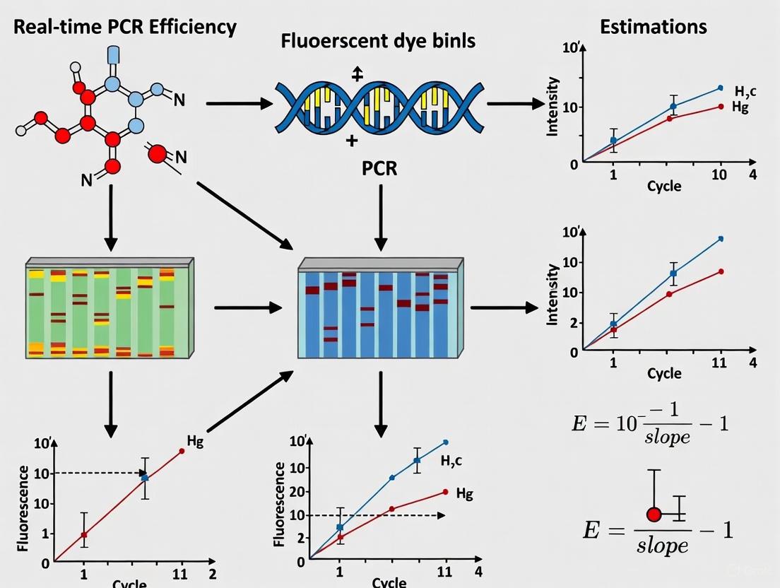
The mathematical relationship between efficiency and quantification becomes evident when examining the logarithmic form of the PCR equation: Log(N₀) = –Log(E + 1) × Ct + Log(N_t) [1] This equation has the linear form y = mx + b, enabling the creation of standard curves for absolute quantification. The slope of this standard curve relates directly to PCR efficiency through the equation: E = 10^(-1/slope) - 1 [3] [4] [5] A slope of -3.32 corresponds to 100% efficiency, with steeper slopes indicating lower efficiency [2]. This mathematical relationship provides the foundation for the most common method of efficiency estimation in qPCR experiments.

Impact of Efficiency on Quantification Accuracy

The exponential nature of PCR amplification means that small variations in efficiency dramatically affect quantification results. For example, a 0.5 variation in Ct results in a 29-41% miscalculation if E = 2, whereas a 0.05 error in E results in a 53-110% miscalculation after 30 cycles [6]. This sensitivity underscores why precise efficiency determination is not merely optional but essential for reliable qPCR results, particularly in gene expression studies where fold-change calculations directly impact biological interpretations [3].

Table 1: Impact of PCR Efficiency on Quantification Accuracy

Efficiency Value	Theoretical Slope	Impact on N₀ Calculation	Practical Implications
100% (E = 1.0)	-3.32	Baseline (ideal)	Optimal quantification accuracy
90% (E = 0.9)	-3.58	2.1-fold under-estimation at Ct=30	Generally acceptable range
80% (E = 0.8)	-3.87	5.8-fold under-estimation at Ct=30	Questionable reliability
110% (E = 1.1)	-3.10	2.8-fold over-estimation at Ct=30	Indicates potential experimental error

Comparative Analysis of Efficiency Estimation Methods

Standard Curve Method

The standard curve method represents the traditional approach for estimating PCR efficiency. This technique involves preparing a dilution series of known template concentrations, amplifying them in parallel with test samples, and plotting Ct values against the logarithm of initial concentrations [7] [2]. The slope of the resulting linear regression is then used to calculate efficiency using the formula E = 10^(-1/slope) - 1 [3] [4].

While widely used, this method has significant limitations. It assumes that efficiency remains constant across all template concentrations, an assumption frequently violated in practice [7] [3]. A 2024 study demonstrated a decreasing trend in efficiency as DNA concentration increased in most cases, likely due to PCR inhibitors [3]. Additionally, standard curves are labor-intensive, require highly concentrated target material that may not be available, and are prone to errors from pipetting inaccuracies, contamination, and inhibitor effects [2] [8]. Recent research highlights that efficiency varies significantly across different qPCR instruments, further complicating standard curve application [8].

Single-Reaction Kinetic Analysis

Alternative methods estimate efficiency from individual amplification curves, eliminating the need for standard curves. These approaches model the exponential phase of amplification using the equation: R_n = R₀ × (1 + E)ⁿ Where R_n is the fluorescence signal at cycle n, and R₀ is the baseline signal [3]. These methods objectively identify the exponential phase of amplification using statistical approaches, such as analyzing standardized residuals to detect significant deviations from linear baseline fluorescence [7].

A 2003 study proposed a computational method that delimits the beginning of exponential observations in PCR kinetics using separate mathematical algorithms for ground fluorescence, non-exponential, and plateau phases [7]. This single-reaction approach provides results of higher accuracy than serial dilution methods and is sensitive to differences in starting target concentrations while resisting researcher subjectivity [7]. These individual-curve methods are particularly valuable for detecting inhibition or other factors that may affect specific samples differently.

Dilution-Replicate Experimental Design

A hybrid approach termed the "dilution-replicate design" replaces traditional identical replicates with dilution replicates for each test sample [6]. This method performs a single reaction on several dilutions for every test sample, creating individual standard curves without independent efficiency estimation. The design enables global efficiency estimation by fitting all standard curves simultaneously with a slope equality constraint, improving estimation robustness [(citation:2].

This approach offers several advantages: it requires fewer reactions than traditional designs, provides the option to exclude outliers rather than repeating runs, and eliminates the need for separate efficiency estimation or inter-run variation controls [6]. The dilution-replicate method effectively combines elements of both standard curve and single-reaction approaches while addressing some of their respective limitations.

Table 2: Comparison of PCR Efficiency Estimation Methods

Method	Principles	Advantages	Limitations
Standard Curve	Serial dilutions of known standards; slope-derived efficiency	Familiar to most researchers; established workflow	Labor-intensive; assumes constant efficiency; pipetting errors affect accuracy
Single-Reaction Kinetics	Mathematical modeling of exponential phase from individual curves	No standard curves needed; identifies sample-specific issues; high accuracy [7]	Complex calculations; requires specialized software or algorithms
Dilution-Replicate Design	Multiple dilutions per sample with global fitting	Fewer reactions; handles outliers well; no separate efficiency estimation [6]	Still requires dilution series; global efficiency assumption
Visual Assessment	Parallelism of geometric slopes on log-scale amplification plots	No equations; not affected by pipetting errors [2]	Subjective; no numerical efficiency value

Experimental Protocols for Efficiency Determination

Standard Curve Protocol for Efficiency Estimation

The following protocol outlines the steps for determining PCR efficiency using the standard curve method, based on established procedures from multiple studies [2] [3] [4]:

• Template Preparation: Prepare a 5-10 point serial dilution series of known template concentration, typically spanning 6-9 orders of magnitude. Use the same matrix as test samples to maintain consistent background effects.

• qPCR Amplification: Run all dilution points in triplicate or quadruplicate on the same qPCR plate under identical cycling conditions. Include no-template controls to detect contamination.

• Data Collection: Record Ct values for each reaction. Manually set a consistent fluorescence threshold within the exponential phase of all amplifications to ensure comparability [4] [1].

• Standard Curve Construction: Plot mean Ct values against the logarithm of initial template quantities. Perform linear regression analysis to determine the slope and R² value.

• Efficiency Calculation: Calculate PCR efficiency using the formula E = 10^(-1/slope) - 1. Acceptable efficiency typically ranges from 90-110% (slope of -3.1 to -3.6) [5].

For precise efficiency estimation, recent research recommends at least 3-4 qPCR replicates at each concentration to reduce uncertainty, which can reach 42.5% with single replicates [8]. Larger transfer volumes during dilution series preparation also reduce sampling error [8].

Protocol for Single-Reaction Efficiency Estimation

For methods estimating efficiency from individual amplification curves [7]:

• Fluorescence Data Export: Export raw fluorescence data from the qPCR instrument for each reaction.

• Background Phase Identification: Apply linear regression to initial cycles to establish the ground fluorescence phase. Use statistical tests (e.g., studentized residuals) to identify the cycle where fluorescence consistently deviates from background.

• Exponential Phase Modeling: Fit the exponential growth model R_n = R₀ × (1 + E)ⁿ to the identified exponential phase or use sigmoidal modeling of the entire amplification curve [3].

• Parameter Optimization: Iteratively adjust parameters to minimize differences between observed and modeled fluorescence values.

• Efficiency Calculation: For any two cycles (a and b) within the exponential phase, calculate efficiency using E = (R_n,a/R_n,b)^1/(C_a-C_b) - 1 [3].

This method's advantage lies in its ability to detect efficiency variations between samples, which is particularly valuable when inhibitors or other sample-specific factors may affect amplification [7].

Figure 1: Single-Reaction Efficiency Estimation Workflow

Experimental Data on Efficiency Estimation Variability

Method-Dependent Efficiency Variations

Recent comparative studies reveal significant variations in efficiency values depending on the mathematical approach used. A 2024 assessment of 16 genes from Pseudomonas aeruginosa demonstrated that efficiency values differed substantially across mathematical methods [3]. When comparing standard curves to individual-curve approaches, researchers observed that:

• Standard curves yielded efficiency values of approximately 100% in three out of four cases
• Exponential model efficiencies ranged from 1.5-2.79 (50-79%)
• Sigmoidal model efficiencies ranged from 1.52-1.75 (52-75%) [3]

These differences directly impacted normalized expression values, highlighting how methodological choices affect final quantitative results. The study further noted a decreasing trend in efficiency as DNA concentration increased in most cases, suggesting PCR inhibitors may contribute to this observed effect [3].

Inter-Assay Variability in Efficiency Estimation

A comprehensive 2025 study evaluating inter-assay variability of standard curves across 30 independent experiments revealed significant variations even under standardized conditions [4]. Research on seven different virus targets showed:

• All viruses demonstrated adequate efficiency (>90%), but with notable variability between targets
• Norovirus GII showed the highest inter-assay efficiency variability
• SARS-CoV-2 N2 gene exhibited the largest quantitative variability (CV 4.38-4.99%) and the lowest efficiency (90.97%) [4]

This variability persisted despite standardized reagents, conditions, consumables, and operators, supporting the recommendation to include standard curves in every experiment for reliable quantification [4]. These findings align with earlier research showing that efficiency estimation varies significantly across different qPCR instruments, though it remains reproducibly stable on a single platform [8].

Table 3: Experimental Efficiency Variations Across Different Studies

Study Reference	Targets Analyzed	Efficiency Range	Key Variability Findings
DNA 2024 [3]	16 bacterial genes	50-100% depending on method	Efficiency decreases with increasing DNA concentration; method choice significantly impacts quantification
Microorganisms 2025 [4]	7 human viruses	90.97-100%	Significant inter-assay variability despite standardized conditions; target-dependent differences observed
Rutledge & Côté 2003 [1]	2 nested amplicons	~100%	Single well-constructed standard curve provides ±6-21% precision depending on Ct
Ståhlberg et al. 2003 [7]	SRY plasmid DNA	Not specified	Single-reaction method more accurate than serial dilutions; sensitive to starting concentration differences

The Scientist's Toolkit: Essential Reagents and Materials

Table 4: Essential Research Reagents for PCR Efficiency Studies

Reagent/Material	Function in Efficiency Assessment	Implementation Example
SYBR Green Master Mix	Fluorescent detection of amplicon accumulation	Provides consistent reaction background for kinetic analysis [3] [9]
Quantified Standard DNA/RNA	Creates standard curve for absolute quantification	Serial dilutions of purified plasmid or synthetic nucleic acids [4] [1]
High-Purity Water	Diluent for standard curves and sample preparation	Minimizes introduction of inhibitors that affect efficiency [3]
Optical Reaction Plates	Compatible with fluorescence detection systems	Ensure consistent signal capture across all wells [4]
Calibrated Pipetting Systems	Accurate liquid handling for dilution series	Reduces technical variability in standard curve preparation [8]

The PCR kinetic equation N₀ = N_t/(E + 1)^Ct establishes an exponential relationship between efficiency (E) and initial target quantification (N₀). This mathematical foundation explains why precise efficiency determination is critical for accurate qPCR results. Current research demonstrates that no single efficiency estimation method is universally superior; each approach presents distinct advantages and limitations. The standard curve method provides familiarity but suffers from inherent variability and resource intensiveness [8] [4]. Single-reaction kinetics offer sample-specific efficiency but require sophisticated algorithms [7] [3]. Dilution-replicate designs present a balanced approach but still necessitate template dilution [6].

For researchers and drug development professionals, these findings underscore the importance of methodological transparency in qPCR experiments. Efficiency should not be treated as a constant but as a variable parameter that requires empirical determination and reporting. As the scientific community moves toward more rigorous quantitative standards, understanding the nuances of the PCR kinetic equation and its implementation remains fundamental to generating reliable, reproducible molecular data that advances both basic research and clinical applications.

In quantitative Polymerase Chain Reaction (qPCR), the amplification efficiency (E-value) is not merely a technical parameter but the foundational pillar upon which reliable quantification is built. It represents the fold increase in amplified product during each cycle of the PCR reaction, with a theoretical maximum of 2 (or 100% efficiency), indicating perfect doubling of the target sequence every cycle [10] [2]. Despite two decades of efforts by the qPCR community to promote standardization, most reported qPCR results remain grossly biased due to improper efficiency handling [10]. Inaccurate E-values initiate a cascade of computational errors that propagate through subsequent analysis, ultimately distorting biological conclusions, compromising diagnostic accuracy, and undermining the reproducibility of scientific research [11]. This review systematically evaluates the sources and impacts of efficiency miscalculation and compares modern methodologies for its accurate determination, providing researchers with a framework for robust nucleic acid quantification.

The Mathematical Cascade: How Efficiency Errors Distort Quantification

The Core Kinetic Equation of PCR

The entire quantitative framework of qPCR rests upon the kinetic equation of PCR:

N_C = N₀ × E_C

Where N_C is the number of amplicons after cycle C, N₀ is the initial target quantity, and E is the amplification efficiency [10]. Through mathematical rearrangement to calculate the initial target quantity (N₀ = N_C/E_C), it becomes evident that efficiency (E) is an exponent in the calculation. Consequently, even minor inaccuracies in E-value estimation become dramatically amplified through this exponential relationship, leading to significant miscalculations of initial target concentration [10] [11].

Table 1: Impact of Efficiency miscalculation on Quantitative Results

True Efficiency	Assumed Efficiency	Reported Quantity vs. True Quantity	Fold Error after 30 Cycles
85% (1.85)	100% (2.00)	Underestimated	5.9-fold
95% (1.95)	100% (2.00)	Underestimated	1.7-fold
105% (2.05)	100% (2.00)	Overestimated	2.1-fold
110% (2.10)	100% (2.00)	Overestimated	4.1-fold

Efficiency in Relative Expression Analysis (ΔΔCq Method)

The popular ΔΔCq method for relative gene expression quantification relies critically on the assumption of perfect, equal efficiency between target and reference gene assays [2]. When this assumption is violated, the mathematical simplification that makes ΔΔCq calculation convenient fails. The standard equation:

Relative Quantity = 2^-ΔΔCq

implicitly sets efficiency at 2 (100%) for all assays [2]. A modified equation accounts for varying efficiencies:

Uncalibrated Quantity = (E_target^-Cttarget)/(E_norm^-Ctnorm)

This correction is essential when target and reference genes amplify with different efficiencies, as failure to apply it introduces systematic errors that render fold-change calculations biologically meaningless [2] [11].

Methodological Comparison: Approaches for Efficiency Determination

Standard Curve Method

The traditional approach for efficiency determination employs a serial dilution series of a known template to generate a standard curve. The slope of the plot of Cq versus log(quantity) relates to efficiency through the equation:

E = 10^-1/slope

A slope of -3.32 corresponds to 100% efficiency [2]. While theoretically sound, this method is notoriously prone to practical errors.

Table 2: Comparison of Efficiency Estimation Methods

Method	Principle	Requirements	Advantages	Limitations
Standard Curve	Linear regression of Cq vs. dilution series	5-7 dilution points, replicates	Familiar, wide dynamic range	Prone to dilution errors, inhibitor effects [2]
Visual Assessment	Parallelism of logarithmic amplification curves	Multiple assays on same plate	No standard curve, identifies inhibition	Subjective, no numerical output [2]
Single-Reaction (LRE)	Fit to logistic model describing efficiency decay	Sufficient cycles in growth phase	No dilutions, accounts for efficiency decline	Requires sophisticated fitting algorithms [12]
Digital PCR	Absolute quantification via Poisson statistics	dPCR platform, partitioning	No standard curve, highest precision	Higher cost, limited throughput [13] [14]

Single-Reaction Efficiency Estimation

Advanced computational methods now enable efficiency estimation from individual amplification curves, eliminating need for standard curves. These approaches model the entire amplification process, accounting for the characteristic decline in efficiency as reagents become limiting. The Logistic Model (LRE) has demonstrated particular promise, producing a parameter E₀ that represents efficiency in the baseline region and agrees closely with calibration-based estimates [12]. Proper implementation requires fitting the raw fluorescence data to a model combining baseline and signal components, typically requiring four to six adjustable parameters in a nonlinear least-squares fit [12]. Statistically, the common practice of "baselining" - separately estimating and subtracting baseline fluorescence before analysis - increases the dispersion of efficiency estimates by approximately 75%, equivalent to tripling the number of reactions needed for equivalent precision [12].

Digital PCR: An Efficiency-Independent Alternative

Digital PCR (dPCR) represents a paradigm shift in nucleic acid quantification by providing absolute quantification without reliance on amplification efficiency or standard curves [13] [14]. Through partitioning of the reaction mixture into thousands of nanoscale reactions, dPCR enables binary endpoint detection (positive/negative) and application of Poisson statistics to calculate absolute template concentration [13]. Recent comparative studies demonstrate dPCR's superior accuracy, particularly for high viral loads of influenza A, influenza B, and SARS-CoV-2, showing greater consistency and precision than Real-Time RT-PCR [13]. This technology eliminates the cascading effects of efficiency miscalculation by circumventing the entire efficiency-based quantification framework.

dPCR Quantification Workflow

Experimental Protocols for Robust Efficiency Determination

Dilution-Replicate Design for Efficiency Estimation

An efficient experimental design alternative to traditional replication uses dilution-replicates instead of identical replicates. In this approach, a single reaction is performed on several dilutions for every test sample, similar to standard curve design but without replicates at each dilution [6]. This design enables simultaneous estimation of both PCR efficiency and initial target quantity through the relationship:

Cq = -log(d)/log(E) + log(T/Q(0))/log(E)

Where d is the dilution factor, E is efficiency, T is threshold fluorescence, and Q(0) is initial quantity [6]. This approach provides inherent quality control, as outliers at extreme dilutions can be identified and excluded without compromising the entire dataset.

One-Point Calibration with Efficiency Correction

For absolute quantification in diagnostic applications, the recommended approach combines a single undiluted calibrator with known target concentration and efficiency values derived from the amplification curves of both calibrator and unknown samples [11]. This method avoids the dilution errors and matrix effects that confound traditional standard curves while still providing efficiency-corrected results essential for meaningful biological interpretation and diagnostic accuracy [11].

Cascading Effects of Inaccurate E-Values

The Scientist's Toolkit: Essential Reagents and Materials

Table 3: Key Research Reagent Solutions for qPCR Efficiency Analysis

Reagent/Material	Function	Considerations for Efficiency
TaqMan Gene Expression Assays	Predesigned primer-probe sets with guaranteed 100% efficiency	Eliminates efficiency estimation burden [2]
Digital PCR Plates/Cartridges	Nanoscale partitioning for absolute quantification	Bypasses efficiency concerns [13] [14]
Standard Curve Reference Material	Known concentration template for efficiency calibration	Requires verification of matrix matching [11]
Inhibitor-Resistant Master Mix	Enhanced polymerase chemistry tolerant to sample inhibitors	Prevents efficiency depression from sample matrix [15]
Nucleic Acid Purification Kits	Remove PCR inhibitors from sample preparations	Maintains optimal reaction efficiency [15]

Accurate determination of PCR efficiency is not an optional refinement but a fundamental requirement for biologically meaningful qPCR results. The cascading effects of inaccurate E-values exponentially amplify through subsequent calculations, rendering quantitative interpretations unreliable. While traditional standard curve methods remain prevalent, they are susceptible to multiple confounding factors including dilution errors, inhibitor effects, and matrix mismatches [2] [11]. Emerging single-reaction estimation methods, particularly those based on logistic models of the entire amplification curve, offer promising alternatives that avoid these pitfalls while providing efficiency values that closely align with calibration-based estimates [12]. For applications demanding the highest possible precision, digital PCR represents the ultimate solution by eliminating efficiency dependence altogether through absolute quantification based on Poisson statistics [13] [14]. As qPCR continues to play a critical role in basic research, diagnostic applications, and drug development, researchers must prioritize proper efficiency determination and correction to ensure the validity and reproducibility of their conclusions. The MIQE (Minimum Information for Publication of Quantitative Real-Time PCR Experiments) guidelines should be extended to explicitly require reporting of both the methods used to determine PCR efficiency and the calculations used to derive reported target quantities [11].

Quantitative Polymerase Chain Reaction (qPCR) is a cornerstone technique in molecular biology for quantifying nucleic acids. Its reliability, however, hinges on a critical parameter: amplification efficiency [16]. Amplification efficiency refers to the rate at which a target DNA sequence is duplicated during each PCR cycle. The ideal, theoretical maximum is 100% efficiency, meaning the number of DNA molecules doubles perfectly with every cycle (a doubling factor of 2.0) [15]. In practice, a benchmark of 90–110% efficiency is widely considered acceptable for a robust and reliable assay [17] [15] [16]. This range corresponds to a standard curve slope between -3.58 and -3.10 [15]. Efficiency outside this optimal window can lead to significant inaccuracies in quantification, misrepresenting the actual amount of the target sequence in the original sample [6]. This article explores the technical underpinnings of this benchmark and investigates the common experimental factors that cause deviations, thereby bridging the gap between the ideal and the real in qPCR experimentation.

The 90-110% Efficiency Benchmark Explained

The 90-110% efficiency range is not an arbitrary guideline but a practical standard grounded in the mathematical relationship between efficiency and quantification accuracy. The calculation of efficiency is typically derived from the slope of a standard curve generated from a serial dilution of a known template [15] [4]. The formula Efficiency = [10^(-1/slope)] - 1 links the slope directly to the reaction's performance [4].

A reaction with 100% efficiency (-3.32 slope) perfectly doubles each cycle, ensuring that the difference in quantification cycle (Cq) values between successive samples in a 2-fold dilution series is exactly 1 [17]. This precision is crucial for distinguishing small concentration differences. As efficiency decreases, the ability to discriminate between 2-fold dilutions diminishes unless the standard deviation of Cq values is very low (≤ 0.167) [17]. The 90-110% benchmark represents a balance where the impact of minor efficiency variations on final quantification remains manageable for most research purposes, ensuring that the fluorescent signal is directly proportional to the initial DNA concentration over the assay's dynamic range [16].

Furthermore, this acceptable range is vital for comparing results across different reactions or laboratories. As highlighted by ThermoFisher, "Ct values from PCR reactions run under different conditions or with different reagents cannot be compared directly" [17]. Adhering to a common efficiency benchmark helps normalize these variables, promoting reproducibility and data integrity in line with the MIQE (Minimum Information for Publication of Quantitative Real-Time PCR Experiments) guidelines [16] [18].

Common Causes of Efficiency Deviations

Deviations from the ideal efficiency range are common in practice and stem from a variety of factors related to reaction chemistry, sample quality, and procedural execution.

Causes of Efficiency Below 90%

• Suboptimal Primer Design: This is a primary cause of poor efficiency. Issues such as primer-dimer formation, self-complementarity (hairpins), or inappropriate melting temperatures (Tm) can severely hinder primer-template annealing and extension, leading to inefficient amplification [15].
• Insufficient Reaction Component Concentration: The concentration of key reagents, including primers, probes, MgCl₂, or dNTPs, may be too low, preventing the polymerase from functioning at its maximum capacity [15].
• Sample Quality and Purity: The presence of polymerase inhibitors in the sample is a major culprit. Common contaminants carried over from nucleic acid isolation steps include ethanol, phenol, and SDS [15]. Other inhibitors like heparin, hemoglobin, and polysaccharides can also bind to or inactivate the polymerase enzyme [15].

Causes of Efficiency Exceeding 110%

While less intuitive, efficiencies significantly above 100% are almost always indicative of underlying problems, rather than a "super-efficient" reaction.

• Presence of PCR Inhibitors: This is the main reason for inflated efficiency values. When inhibitors are present in more concentrated samples, they cause a delay in the Cq value, meaning more cycles are needed for detection than should be. As the sample is diluted, the inhibitors are also diluted, reducing their effect and causing the Cq values to shift closer to the expected values. This flattens the standard curve, resulting in a shallower slope and a calculated efficiency of over 100% [15].
• Fluorescent Background or Non-Specific Amplification: When using intercalating dyes, the formation of primer-dimers or the amplification of unspecific products can generate a fluorescent signal that is not solely from the target amplicon. This artificial inflation of the background signal can distort the early, baseline phase of the amplification plot, leading to an incorrect calculation of efficiency [15].
• Pipetting Errors and Inaccurate Dilution Series: Inconsistent technique when preparing the standard curve dilutions can create a curve that does not accurately reflect the true logarithmic relationship between concentration and Cq, directly impacting the slope and the resulting efficiency calculation [15].

Table 1: Summary of Common Causes for qPCR Efficiency Deviations

Deviation Type	Primary Causes	Underlying Mechanism
Low Efficiency (<90%)	Suboptimal primer design [15]	Poor annealing/extension; primer-dimer formation
	Non-optimal reagent concentrations [15]	Limiting components for polymerase activity
	Presence of polymerase inhibitors [15]	Enzyme inactivation or binding
High Efficiency (>110%)	PCR inhibition in concentrated samples [15]	Flattened standard curve due to delayed Cq in high-concentration samples
	Unspecific amplification or primer dimers [15]	Dye-based fluorescence not solely from target
	Pipetting errors; inaccurate dilutions [15]	Incorrect standard curve slope

Methodologies for Efficiency Estimation and Validation

Accurately determining qPCR efficiency is a prerequisite for validating any assay. The following experimental protocols are standard in the field.

Standard Curve Method

This is the most common approach for determining amplification efficiency.

• Serial Dilution Preparation: A sample with a known concentration of the target nucleic acid (e.g., a plasmid, PCR product, or synthetic oligonucleotide) is serially diluted. A minimum of 5 logs of template concentration is recommended for a rigorous evaluation, as a wider range reduces the artifact in efficiency calculation [17]. Each dilution is typically run in a minimum of 3 replicates.
• qPCR Run: The dilution series is amplified using the qPCR protocol under validation.
• Data Analysis: The mean Cq value for each dilution is plotted against the logarithm of its initial concentration. A linear regression trendline is fitted to the data points. The slope of this line is used to calculate efficiency using the formula: E = [10^(-1/slope)] - 1 [15] [4].
• Quality Assessment: The linear dynamic range and the coefficient of determination (R²) must be evaluated. An R² value >0.99 indicates a strong linear relationship and good predictability [17]. The linear range is the span of concentrations where the signal is directly proportional to the input [16].

Alternative Experimental Designs

Alternative methods can improve efficiency estimation while optimizing resource use. The dilution-replicate design proposes using several dilutions of every test sample instead of identical replicates. This design inherently generates a standard curve for each sample, allowing for direct efficiency estimation without independent curves and providing the option to exclude outliers from specific dilutions [6]. The data from all samples can be fit with a constraint of slope equality to derive a globally estimated PCR efficiency, which benefits from a higher degree of freedom and can be more robust against individual Cq errors [6].

A Practical Workflow for Efficiency Troubleshooting

The following diagram maps a logical pathway for diagnosing and correcting sub-optimal qPCR efficiency.

The Scientist's Toolkit: Essential Reagents and Materials

Successful qPCR assay development and validation require specific, high-quality reagents and materials. The following table details key components used in the experiments and methodologies cited in this guide.

Table 2: Key Research Reagent Solutions for qPCR Validation

Reagent / Material	Function / Application	Example Use-Case
TaqMan Fast Virus 1-Step Master Mix [4]	An optimized ready-to-use mix for reverse transcription and qPCR, minimizing handling and variability.	Used in a 30-experiment study on standard curve variability for virus quantification in wastewater [4].
GeneProof PathogenFree DNA Isolation Kit [19]	For efficient extraction of inhibitor-free DNA from complex clinical samples like tissue biopsies.	Used for DNA extraction from pediatric gastric biopsies prior to H. pylori detection via real-time PCR and HRM [19].
Quantitative Synthetic RNA (from ATCC) [4]	Provides a stable, standardized material for generating consistent standard curves and determining assay limits.	Served as an exogenous positive control and standard for 30 independent RT-qPCR standard curve experiments for 7 different viruses [4].
QIAcuity Digital PCR System [13]	A nanowell-based dPCR platform for absolute quantification without a standard curve, used for method comparison.	Employed in a comparative study with RT-qPCR for quantifying respiratory viruses (Influenza, RSV, SARS-CoV-2) [13].
Seegene Allplex Respiratory Panel [13]	A multiplex Real-Time RT-PCR kit for the simultaneous detection of multiple respiratory pathogens.	Used for the initial detection and stratification of viral loads in respiratory samples in a dPCR vs. RT-qPCR comparison study [13].

The 90-110% efficiency benchmark is a pragmatic and scientifically grounded target that ensures the quantitative reliability of qPCR data. While the ideal of 100% efficiency is a valuable guide, real-world experimental conditions—ranging from primer design and reagent quality to the insidious presence of inhibitors—frequently cause deviations. Understanding these causes is the first step toward remediation. By employing rigorous validation methods like the standard curve, adhering to troubleshooting workflows, and utilizing appropriate reagents and controls, researchers can diagnose and correct efficiency problems. This disciplined approach bridges the gap between theoretical ideals and practical reality, ensuring that qPCR remains a robust and trustworthy tool for genetic quantification in research and diagnostics.

The quantitative polymerase chain reaction (qPCR) amplification curve is a fundamental visual representation of the DNA amplification process, charting the accumulation of fluorescence over consecutive cycles. Accurately identifying its distinct phases—ground, exponential, and plateau—is not merely an analytical exercise but a critical prerequisite for reliable gene quantification. The entire premise of qPCR quantification rests on establishing a quantitative relationship between the initial amount of target nucleic acid and the data gathered during the exponential phase [20]. Misidentification of these phases can lead to incorrect efficiency calculations and substantially skewed results, undermining the validity of any downstream analysis [21] [3]. This guide objectively compares the performance of different curve analysis methods, providing a framework for researchers to evaluate these approaches within the broader context of PCR efficiency estimation research.

Phase Characteristics and Quantitative Signatures

Each phase of the qPCR amplification curve possesses unique characteristics and quantitative signatures that researchers must recognize for accurate analysis. The following table summarizes the key attributes of each phase.

Table 1: Characteristics of qPCR Amplification Curve Phases

Phase	Cycle Range	Fluorescence Trend	PCR Efficiency	Data Utility for Quantification
Ground (Linear/Baseline)	Early cycles (typically 1-15) [22]	At or near background level; little change [21]	Not applicable	Fluorescence establishes background level; quantification unreliable [23]
Exponential (Log-Linear)	Varies by initial template concentration	Rapid, exponential increase [20]	Constant and maximal [22]	Primary phase for reliable quantification [20] [3]; fluorescence is proportional to starting template [24]
Transitional	Follows exponential phase	Increase rate decreases as reagents become limiting [21]	Declining from maximum	Not suitable for quantification due to variable efficiency [21]
Plateau	Late cycles (e.g., 30-40)	Fluorescence stabilizes; no significant increase [20] [23]	Near zero; reaction stops [20]	Not useful for data calculation [20]; endpoint fluorescence is not representative of initial template [21]

The progression through these phases is visually represented in the following amplification curve diagram.

Diagram 1: The four distinct phases of a typical qPCR amplification curve, showing the transition from background fluorescence through exponential growth to reaction saturation.

Experimental Protocols for Phase Identification

Standard Curve Method for Efficiency Determination

The standard curve method is a foundational approach for quantifying PCR efficiency and validating that the threshold for quantification is set within the exponential phase [20].

• Preparation of Standard Dilutions: Create a serial dilution series of a known concentration of target DNA or RNA. Typically, five to six log-fold dilutions are prepared (e.g., 1:10, 1:100, 1:1000) [23] [4].
• qPCR Run: Amplify all standard dilutions and unknown samples in the same qPCR run, ideally using triplicate technical replicates for each dilution point [23].
• Data Collection and Ct Determination: The qPCR instrument software records the fluorescence and calculates the Cycle threshold (Ct) for each reaction, which is the cycle number at which the fluorescence crosses a defined threshold [20].
• Standard Curve Plotting and Efficiency Calculation: Plot the log of the known starting concentration of each standard dilution against its mean Ct value. Perform linear regression to obtain the slope of the trendline. The PCR efficiency is then calculated using the formula: Efficiency (%) = (10⁻¹/ˢˡᵒᵖᵉ - 1) × 100 [3] [23] [4]. Optimal efficiency falls between 90-110% [23], corresponding to a slope of -3.6 to -3.1.

Individual Sample Efficiency Analysis with LinRegPCR

For a method that foregoes standard curves and calculates efficiency from the amplification profile of each sample, the LinRegPCR software provides a robust protocol [24] [22].

• Baseline Correction: The software performs an automated, user-independent baseline subtraction. Unlike instrument software that often uses the noisy ground phase cycles, LinRegPCR uses an iterative approach to determine a baseline value that results in the most data points forming a straight line in a log(fluorescence) versus cycle number plot [22].
• Identification of the Exponential Phase: The start of the exponential phase is identified as the first cycle with a continuous increase in fluorescence. The end is defined by the Second Derivative Maximum (SDM), the cycle where the increase in fluorescence begins to decrease, marking the transition into the plateau phase [22].
• Efficiency Calculation per Assay: The PCR efficiency for each reaction is determined from the slope of the exponential phase (a minimum of three consecutive cycles). To reduce variability, the efficiencies of all reactions for the same target are averaged, yielding a mean PCR efficiency per assay [22] [23].
• Setting a Common Quantification Threshold: A single fluorescence threshold is set within the exponential phase of all reactions, ensuring that Cq values are directly comparable across the entire run [22].

Comparative Performance of Analysis Methods

Different mathematical approaches for modeling amplification curves and estimating efficiency can yield varying results, directly impacting DNA quantification and gene expression analysis [3].

Table 2: Comparison of qPCR Efficiency Estimation Methods

Method	Principle	Efficiency Range Reported	Impact on Quantification	Best Use Cases
Standard Curve	Linear regression of log(concentration) vs. Ct from diluted standards [3]	Typically >90% [4]	Assumes constant efficiency for all samples; potential overestimation [3]	Absolute quantification; clinical viral load testing [20] [4]
Exponential Model (Individual Curves)	Fitting the exponential phase of individual amplification curves [3]	65-90% is common [21]; 50-79% in experimental data [3]	Accounts for sample-to-sample variation; more precise relative quantification [24]	High-precision gene expression studies; when standard curves are impractical [24] [22]
Sigmoidal Model	Modeling the entire amplification curve (baseline, exponential, plateau) [3]	52-75% in experimental data [3]	Considers the full reaction kinetics; may better handle suboptimal reactions	Research with variable sample quality; comprehensive kinetic analysis [3]
2-ΔΔCt (Livak)	Assumes ideal doubling efficiency (100%) for all reactions [3] [23]	Fixed at 100% (not calculated)	Can produce significant inaccuracies if true efficiency deviates from 100% [3]	Rapid screening only when target and reference genes are validated to have near-perfect efficiency [23]

The Scientist's Toolkit: Essential Reagent Solutions

Successful interpretation of amplification curves relies on the quality of reagents and materials used in the qPCR workflow.

Table 3: Essential Research Reagents and Materials for qPCR

Reagent/Material	Function	Considerations for Curve Analysis
SYBR Green I Master Mix	DNA-binding dye that fluoresces when bound to double-stranded DNA [20]	Dye chemistry can produce higher background in baseline phase compared to probe-based methods [22]. Use of a passive reference dye (ROX) allows for normalization (Rn) to minimize well-to-well variation [23].
Hydrolysis Probes (TaqMan)	Sequence-specific probes with a fluorophore and quencher; fluorescence increases upon cleavage [20]	Provides higher specificity, reducing background signal from non-specific products. Baseline fluorescence can be higher (up to 10% of final signal) due to incomplete quenching [22].
Primers	Short DNA sequences that define the region to be amplified [20]	Critical for reaction efficiency. Poor design (e.g., primer-dimer formation) can distort the baseline and exponential phases, leading to inaccurate Cq and efficiency values [24].
Hot-Start DNA Polymerase	Enzyme engineered to reduce activity at lower temperatures, preventing non-specific amplification [9]	Minimizes primer-dimer and other non-specific products in early cycles, resulting in a cleaner baseline and more reliable transition into the true exponential phase [9].
Commercial Lysis Buffers (e.g., SIL-B)	For direct PCR from crude samples (e.g., blood) without nucleic acid purification [9]	Reduces processing time but may introduce PCR inhibitors that depress reaction efficiency, flattening the exponential phase and increasing Cq values [9].

The precise identification of the ground, exponential, and plateau phases in a qPCR amplification curve is a cornerstone of reliable molecular quantification. As demonstrated, the choice of analysis method—whether standard curve, exponential, or sigmoidal modeling—significantly impacts the calculated PCR efficiency and final quantitative results. Researchers must be aware that efficiency is not an abstract value but a kinetic parameter directly derived from the exponential phase of the curve. For most applications requiring high accuracy, particularly in gene expression analysis or diagnostic validation, methods that calculate efficiency from individual sample curves, such as LinRegPCR, provide superior reproducibility and minimize the influence of inter-assay variability. Ultimately, robust experimental design, combined with a critical approach to curve interpretation, ensures that qPCR data remains a gold standard in quantitative molecular biology.

The cycle quantification (Cq) value, representing the PCR cycle at which a target amplicon is first detected, serves as the foundational data point in quantitative real-time PCR (qPCR) analysis. While this metric provides a convenient starting point for quantification, relying solely on Cq values without proper context of amplification efficiency introduces substantial risks in data interpretation. The prevailing assumption that Cq values directly and consistently correlate with initial template quantity across samples and experiments often fails in practice due to numerous technical and biological variables. This analysis examines the critical limitations of Cq-centric approaches and evaluates methodological frameworks for robust efficiency estimation, providing researchers with strategies to overcome these foundational pitfalls in molecular quantification.

The Critical Role of Amplification Efficiency in qPCR Quantification

Fundamental Relationship Between Cq and Efficiency

In qPCR, the relationship between the Cq value and the initial template quantity is mathematically described by the exponential amplification equation: Q = Q₀ × (1+E)^Cq, where Q represents the product quantity at the Cq value, Q₀ is the initial template quantity, and E is the amplification efficiency (values from 0 to 1, or 0% to 100%) [25] [2]. This equation forms the basis for all subsequent quantification methods. When efficiency is 100% (E=1), the template doubles every cycle, and the relationship becomes Q = Q₀ × 2^Cq. The inverse relationship means that higher initial template concentrations result in lower Cq values, while lower concentrations yield higher Cq values [25].

The critical importance of efficiency becomes apparent when considering that a slight variation in efficiency exponentially impacts calculated template quantities over multiple cycles. For a Cq of 20, the quantities resulting from 100% versus 80% efficiency differ by approximately 8.2-fold [2]. This dramatic effect underscores why accurate efficiency determination is paramount for reliable quantification.

Efficiency Estimation Methods and Their Limitations

The standard curve method remains the most widely accepted approach for estimating PCR efficiency [26]. This method involves creating a dilution series of a template with known relative concentrations, then plotting the Cq values against the logarithm of the concentrations. The efficiency is derived from the slope of the resulting line using the equation: E = 10^(-1/slope) - 1 [26] [2]. For a 10-fold dilution series, a slope of -3.32 corresponds to 100% efficiency [2].

However, this method contains inherent limitations. Errors in standard curve slopes are common due to inhibitors, contamination, pipetting inaccuracies, and dilution point mixing problems [2]. These errors can theoretically produce slopes suggesting greater than 100% efficiency, even though geometric efficiency cannot actually exceed 100% [2]. The visual assessment method offers an alternative approach by comparing geometric amplification slopes across assays. Parallel slopes suggest similar efficiencies, while non-parallel slopes indicate varying efficiencies [2].

Table 1: Impact of Amplification Efficiency Errors on Quantification

Efficiency Error	Impact on Calculated Quantity	Impact After 30 Cycles
5% overestimation	53% overestimation [6]	Substantial overestimation
5% underestimation	29% underestimation [6]	Substantial underestimation
20% lower efficiency	8.2-fold difference at Cq 20 [2]	Dramatic miscalculation

Critical Limitations of Cq-Value-Centric Analysis

Platform-Dependent Variability and Lack of Commutability

Cq values demonstrate significant variability across different qPCR platforms and laboratory setups, fundamentally limiting their direct comparability. A compelling example comes from SARS-CoV-2 testing, where studies revealed different Ct value thresholds correlated with clinical outcomes across different test platforms, even after controlling for other factors [27]. This platform-dependent variability means that Cq values obtained from one system cannot be directly compared to those from another, complicating cross-study comparisons and meta-analyses.

The interquartile ranges of Cq values between different patient groups and testing platforms can overlap by 20-50%, substantially reducing the discriminatory power for individual clinical decision-making [27]. This variability stems from multiple technical sources including different specimen collection devices, nucleic acid extraction methods, genomic targets, and RT-PCR chemistries [27]. Consequently, professional organizations like the Infectious Diseases Society of America (IDSA) and the Association for Molecular Pathology (AMP) jointly recommend against using Cq values for individual patient care decisions with qualitative tests [27].

Unaccounted Statistical Uncertainty and False Positive Rates

A fundamentally overlooked problem in conventional Cq value analysis is the systematic underestimation of statistical uncertainty when amplification efficiency estimates are treated as fixed values rather than distributions. Current efficiency-adjusted ΔΔCq methods typically disregard the uncertainty of the estimated efficiency, effectively assuming infinite precision in efficiency estimation [28]. This statistical oversight produces overly optimistic standard errors, artificially narrow confidence intervals, and deflated p-values that ultimately increase Type I error rates beyond expected significance levels [28].

The consequences of this statistical omission are particularly pronounced in validation studies where false positive control is paramount. When efficiency is determined with inadequate precision, the resulting inference on ΔΔCq values becomes dangerously anti-conservative, potentially leading to erroneous conclusions about differential expression [28]. Proper accounting of efficiency uncertainty through methods like the statistical delta method, Monte Carlo integration, or bootstrapping is necessary to maintain appropriate false positive rates, especially when efficiency estimates are based on limited dilution series or technical replicates [28].

Statistical Uncertainty Propagation in Cq Value Analysis

Template Sequence-Specific Bias in Multi-Template PCR

In multi-template PCR applications—essential for metabarcoding, microbiome studies, and DNA data storage—sequence-specific amplification efficiencies create substantial quantification bias independent of initial template abundance. Recent research utilizing deep learning models has demonstrated that specific sequence motifs adjacent to priming sites significantly impact amplification efficiency, challenging long-standing PCR design assumptions [29].

This phenomenon manifests as progressively skewed coverage distributions during amplification, where sequences with disadvantaged amplification efficiencies become severely underrepresented [29]. Remarkably, this bias persists even when controlling for GC content, suggesting previously unrecognized sequence-specific factors influence amplification efficiency [29]. Approximately 2% of random sequences demonstrate severely compromised amplification efficiencies as low as 80% relative to the population mean, resulting in their effective disappearance from sequencing data after 60 cycles [29].

The identification of adapter-mediated self-priming as a major mechanism causing low amplification efficiency provides mechanistic insight into this bias [29]. This sequence-dependent efficiency variation fundamentally undermines the assumption that Cq values or read counts directly reflect initial template abundances in multi-template applications, necessitating computational correction or specialized experimental designs.

Experimental Design Considerations for Robust Efficiency Estimation

Optimal Standard Curve Construction

Robust efficiency estimation requires carefully constructed standard curves with appropriate replication and dilution schemes. Evidence-based recommendations indicate that precise efficiency estimation requires standard curves with at least 3-4 qPCR replicates at each concentration [26]. Furthermore, using larger transfer volumes (e.g., 2-10μL) during serial dilution preparation reduces sampling error and enables calibration across wider dynamic ranges [26].

The ideal standard curve structure for accurate efficiency assessment consists of 7 points with a 10-fold dilution series [2]. However, practical constraints often necessitate modifications. The dilution-replicate experimental design offers an efficient alternative by performing single reactions on several dilutions for each test sample rather than multiple identical replicates [6]. This approach simultaneously estimates both PCR efficiency and initial quantity while providing built-in outlier identification through multiple dilution points [6].

Table 2: Recommended Experimental Designs for Efficiency Estimation

Parameter	Traditional Approach	Dilution-Replicate Design	Evidence Source
Technical Replicates	3 identical replicates per sample	Multiple dilutions per sample (no identical replicates)	[6]
Dilution Points	4-5 points for 2-3 independent samples	3+ dilution points per sample	[6] [2]
Minimum Replicates	3-4 qPCR replicates per concentration	Single reactions per dilution point	[26]
Template Choice	Purified PCR product (risk of side reactions)	cDNA library or genomic DNA with target sequence	[26]
Volume Transfer	Not specified	2-10μL to reduce sampling error	[26]

Template Selection and Quality Considerations

Template choice significantly impacts efficiency estimates and their applicability to experimental samples. Purified PCR products, while convenient, often promote side reactions due to their short length and fail to reflect the effect of flanking sequences that may interfere with PCR through structural interactions [26]. For gene expression analysis, cDNA libraries provide long template molecules with representative secondary structures that better mimic experimental conditions [26]. For DNA quantification, genomic DNA or plasmids containing the gene of interest serve as appropriate standards, preferably after excising a fragment containing the target sequence to eliminate interfering supercoiling effects [26].

Sample quality assessment remains crucial, as inhibitors present in the sample matrix can substantially reduce apparent efficiency. Proper validation includes testing for inhibition through RNA or DNA spikes or serial dilution analysis [26]. Inhibition often manifests as deviation from linearity in concentrated samples, potentially causing unrealistic efficiency estimates exceeding 100% if these points are erroneously included in linear regression [26].

Template Selection and Experimental Design Workflow

Advanced Methodological Approaches and Computational Solutions

Linear Mixed Models for Uncertainty Propagation

Linear mixed effects models (LMMs) provide a statistical framework that simultaneously estimates the uncertainty of both efficiency and Cq values, properly accounting for technical and sample-level variability [28]. This approach enables correct propagation of efficiency estimation error into final ΔΔCq estimates, maintaining appropriate false positive rates in hypothesis testing [28]. While the concept of using LMMs in qPCR analysis is not novel, their application combined with statistical methods like the delta method, Monte Carlo integration, or bootstrapping to handle efficiency uncertainty represents an important methodological advancement [28].

The modified ΔΔCq equation incorporating efficiency terms takes the form: Uncalibrated Quantity = (etarget^(-Cttarget))/(enorm^(-Ctnorm)), where e represents geometric efficiency and Ct represents the threshold cycle for target and normalizer assays [2]. This formulation allows for differing efficiencies between target and reference genes, addressing a common source of bias in traditional ΔΔCq calculations that assume equal, perfect efficiency [2].

Deep Learning for Sequence-Specific Efficiency Prediction

Emerging computational approaches leverage deep learning to predict sequence-specific amplification efficiencies directly from DNA sequence information. Recent research demonstrates that one-dimensional convolutional neural networks (1D-CNNs) can accurately predict amplification efficiencies based solely on sequence features, achieving high predictive performance (AUROC: 0.88, AUPRC: 0.44) [29].

These models, trained on synthetic DNA pools with reliably annotated efficiency values, enable the identification of specific motifs associated with poor amplification and facilitate the design of inherently homogeneous amplicon libraries [29]. The CluMo (Motif Discovery via Attribution and Clustering) interpretation framework identifies problematic sequence motifs adjacent to adapter priming sites, revealing adapter-mediated self-priming as a major mechanism causing low amplification efficiency [29]. This approach reduces the required sequencing depth to recover 99% of amplicon sequences fourfold, offering significant efficiency improvements in multi-template PCR applications [29].

The Scientist's Toolkit: Research Reagent Solutions

Table 3: Essential Reagents and Materials for Robust qPCR Efficiency Estimation

Reagent/Material	Function	Specifications/Quality Controls
TaqMan Gene Expression Assays	Pre-designed, pre-optimized primer-probe sets	>700,000 assays available; guaranteed 100% efficiency [30] [2]
Custom TaqMan Assay Design Tool	Web-based design of custom assays	Superior algorithm for optimal primer-probe design [30]
SYBR Green I Master Mix	Fluorescent DNA binding dye for detection	Requires validation of specificity via melt curve analysis [26]
Standard Curve Templates	Efficiency estimation reference	cDNA library, genomic DNA, or synthetic templates (gBlocks) [26]
DNase Treatment Reagents	gDNA removal from RNA samples	Critical for preventing false positives from contaminating gDNA [30]
Nucleic Acid Quality Assessment Tools	Sample quality verification	Spectrophotometric ratios (A260/A280, A260/A230); RNA integrity number [26]

The limitations of relying solely on Cq values for qPCR quantification stem from multiple sources: efficiency variability across platforms and sequences, unaccounted statistical uncertainty, and template-specific amplification biases. Robust quantification requires moving beyond Cq-centric approaches to incorporate proper efficiency estimation, uncertainty propagation, and sequence-aware design. Methodological frameworks employing linear mixed models, advanced experimental designs, and emerging deep learning approaches offer pathways to overcome these fundamental limitations. As qPCR continues to serve critical roles in both basic research and clinical applications, acknowledging and addressing these foundational pitfalls remains essential for generating reliable, reproducible molecular quantification data.

A Practical Guide to Efficiency Estimation Methods: From Standard Curves to Single-Curve Analysis

In molecular biology, the accuracy of quantitative real-time PCR (qPCR) hinges on a critical component: the standard curve. This method serves as the gold standard for quantifying nucleic acids, providing a reliable benchmark against which the performance of both samples and assays are measured [31]. A gold standard test is defined as the best available diagnostic method under reasonable conditions, against which new tests are compared to gauge their validity [32]. In the context of a broader thesis on evaluating real-time PCR efficiency estimation methods, understanding the construction, interpretation, and limitations of standard curves is fundamental. This guide objectively compares this established methodology with emerging alternatives, such as digital PCR (dPCR), providing the experimental data and protocols researchers and drug development professionals need to make informed methodological choices.

The Fundamental Principles of the qPCR Standard Curve

The qPCR standard curve is a relationship model between the quantification cycle (Cq) values and the logarithm of known, serially diluted template concentrations [8]. This curve enables the conversion of raw Cq values from samples with unknown concentrations into absolute quantities. Its two most critical parameters are the slope and the correlation coefficient (R²).

The PCR efficiency (E) is calculated from the slope of the standard curve using the formula: E = [10^(-1/slope)] - 1 [8]. An ideal reaction with 100% efficiency, where the template doubles perfectly every cycle, has a slope of -3.32. In practice, an efficiency between 90% and 110% (slope between -3.58 and -3.10) is generally considered acceptable. The R² value, ideally >0.99, indicates the linearity and reliability of the curve across the dynamic range.

Building a Robust Standard Curve: Detailed Experimental Protocol

Constructing a precise standard curve requires meticulous attention to each step of the workflow, illustrated below.

Step 1: Preparation of Standard Material

The process begins with a template of known concentration, typically a synthetic oligonucleotide, purified PCR product, or genomic DNA. The initial concentration must be accurately determined using a high-integrity method like spectrophotometry (NanoDrop) or fluorometry (Qubit). This stock solution is then serially diluted, usually in 10-fold steps, to span the entire expected concentration range of the unknown samples, typically covering 5 to 6 orders of magnitude (e.g., from 10^0 to 10^5 copies/µL).

Step 2: qPCR Amplification

Each dilution in the series is amplified by qPCR in a minimum of 3-4 technical replicates to account for random pipetting and instrumentation errors [8]. All reactions must be performed under identical conditions: the same reaction mix, cycling protocol, and on the same instrument plate. The inclusion of a no-template control (NTC) is mandatory to confirm the absence of contamination.

Step 3: Data Analysis and Curve Fitting

The mean Cq value for each standard dilution is plotted against the logarithm of its known concentration. A regression line is fitted to these data points. The slope, y-intercept, and R² value of this line are automatically calculated by the qPCR instrument software. The PCR efficiency is then derived from the slope.

Step 4: Quantification of Unknowns

The Cq values of unknown samples are interpolated from the standard curve to determine their initial concentrations. The reliability of this quantification is directly dependent on the quality and precision of the standard curve.

Key Reagents and Research Solutions

The following table details essential materials and their functions for establishing a reliable qPCR standard curve.

Item Name	Function/Brief Explanation
High-Purity Standard Template	A DNA or RNA fragment of known sequence and concentration. Serves as the absolute reference for quantification.
High-Fidelity DNA Polymerase	Enzyme for amplifying the standard template to ensure minimal introduction of errors during PCR product generation.
qPCR Master Mix	Optimized buffer containing DNA polymerase, dNTPs, salts, and fluorescent dyes (SYBR Green) or probe systems (TaqMan).
Spectrophotometer/Fluorometer	Instrument for accurately quantifying the initial concentration of the standard stock solution.
qPCR Thermocycler	Instrument that performs thermal cycling while monitoring fluorescence in real-time to generate Cq values.

Comparative Performance Data: qPCR vs. Digital PCR

While qPCR is the established workhorse for nucleic acid quantification, digital PCR (dPCR) has emerged as a powerful alternative that eliminates the need for a standard curve. dPCR achieves absolute quantification by partitioning a sample into thousands of individual reactions, counting the positive and negative partitions, and using Poisson statistics to determine the original copy number [13] [31]. The table below summarizes a comparative performance analysis based on recent studies.

Table 1: Comparative analysis of qPCR and dPCR performance characteristics.

Parameter	Real-Time PCR (qPCR)	Digital PCR (dPCR)
Quantification Basis	Relative to standard curve [31]	Absolute count of molecules [31]
PCR Efficiency	Requires precise estimation [8]	Largely independent of efficiency [13]
Precision & Sensitivity	High for moderate to high abundance targets [13]	Superior for low-abundance targets and rare mutations [13] [31]
Susceptibility to Inhibitors	Moderate; can affect Cq values [13]	Lower; partitioning reduces inhibitor effects [13]
Throughput & Cost	High-throughput, cost-effective [31]	Lower throughput, higher cost per sample [13]
Ideal Application	Gene expression, pathogen detection (high titer) [31]	Liquid biopsy, rare allele detection, viral load (low titer) [13] [31]

A 2025 study on respiratory virus diagnostics during the 2023-2024 tripledemic provided concrete data supporting this comparison. The study found that dPCR "demonstrated superior accuracy, particularly for high viral loads of influenza A, influenza B, and SARS-CoV-2," and showed "greater consistency and precision than Real-Time RT-PCR, especially in quantifying intermediate viral levels" [13]. This highlights dPCR's performance advantages in scenarios demanding high precision, though the study notes its routine use is still limited by higher costs and reduced automation compared to qPCR [13].

Interpreting Results and Troubleshooting a Suboptimal Curve

A precise standard curve is the foundation of reliable data. The following diagram outlines the logical process for diagnosing and resolving common issues based on the curve's parameters.

Robust efficiency estimation is not merely academic; it has direct implications for quantitative accuracy. A study on the imprecision of PCR efficiency estimation found that the uncertainty may be as large as 42.5% if a standard curve with only one qPCR replicate is used [8]. This underscores the necessity of using at least 3-4 technical replicates per concentration to reduce this uncertainty and generate a precise efficiency estimate [8]. Furthermore, the estimated PCR efficiency can vary significantly across different qPCR instruments, indicating that a standard curve generated on one platform should not be assumed to be valid on another [8].

The qPCR standard curve remains the gold standard method for nucleic acid quantification due to its robustness, high throughput, and cost-effectiveness. Its proper construction and interpretation, requiring careful dilution series preparation, adequate replication, and critical evaluation of efficiency and linearity, are non-negotiable for generating valid data [8]. However, the emergence of dPCR presents a compelling alternative for applications where absolute quantification without a standard curve, superior precision for low-abundance targets, and reduced susceptibility to inhibitors are paramount [13] [31]. The choice between these technologies is not a matter of one being universally better, but rather depends on the specific requirements of the experiment—weighing the need for throughput and cost against the demand for ultimate sensitivity and precision. As the field of molecular diagnostics advances, the principles of the standard curve continue to underpin the validation of these new technologies, ensuring that the "gold standard" evolves while maintaining its foundational integrity.

In real-time quantitative PCR (qPCR), the accuracy of quantitative results is fundamentally dependent on the amplification efficiency of the assay. The standard curve method provides a robust, widely practiced approach for determining this critical parameter. Amplification efficiency (E) is defined as the fraction of target templates that is amplified during each PCR cycle; an efficiency of 1 (or 100%) represents a perfect doubling of amplicons every cycle [2] [10].

The relationship between the standard curve's slope and PCR efficiency is mathematically codified in the formula E = 10^(-1/slope) - 1 [33] [34]. This guide objectively compares this method against alternative approaches, evaluating its performance based on precision, practical implementation, and applicability within modern molecular research and drug development.

Core Principles: The Slope-Efficiency Relationship

The Mathematical Foundation

The standard curve is generated from a dilution series of a known template quantity. The threshold cycle (Ct) values obtained from these dilutions are plotted against the logarithm of their starting concentrations. The slope of the resulting trendline is the central component for calculating efficiency [34] [35].

• Ideal Scenario: A slope of -3.32 corresponds to a PCR efficiency of 100% [2] [34]. This is derived from the fact that a template doubling every cycle (100% efficiency) should see the Ct value change by -1 for every 2-fold dilution, or by approximately -3.32 for every 10-fold dilution (since log10(2) ≈ 0.301, and 1/0.301 ≈ 3.32).
• Acceptable Ranges: In practice, PCR efficiencies between 90% and 110% (approximately corresponding to slopes between -3.58 and -3.10) are generally considered acceptable for reliable quantification [34] [36]. Efficiencies outside this range can indicate issues with reaction optimization or the presence of inhibitors.

Performance Data and Comparison of Methods

The table below summarizes key performance characteristics and compares the standard curve method to other common approaches for efficiency estimation.

*Table 1: *Comparison of qPCR Efficiency Estimation Methods

Method Feature	Standard Curve with Dilution Series	PCR Efficiency-Based Calculations (e.g., LinReg, DART-PCR)	Assumption of 100% Efficiency (ΔΔCq Method)
Core Principle	Relies on external dilution series to establish Ct-log(quantity) relationship [35].	Calculates efficiency from the exponential phase of individual sample amplification curves [33].	Assumes perfect doubling in every cycle; no experimental determination of actual efficiency [10].
Quantitative Output	Provides a precise efficiency value (E) for the assay [33] [34].	Provides an efficiency value per sample.	Does not provide an efficiency value; it is fixed at 2 (100%).
Key Quality Indicators	Slope (ideal: -3.32) and Coefficient of Determination (R²) (should be >0.99) [34] [16].	Confidence interval of the calculated efficiency.	Not applicable.
Major Advantage	Simple, reliable, and provides routine validation of the methodology [35].	Does not require laborious preparation of a dilution series [33].	Extreme simplicity and low cost; no extra experiments needed.
Major Disadvantage	Requires additional labor, cost, and a suitable sample for the dilution series [2].	The "black-box" nature of algorithms and sensitivity to baseline setting can affect results [10].	Introduces significant bias if the true assay efficiency deviates from 100%, leading to inaccurate quantification [10].
Impact of Inhibitors	Can be detected by a sub-optimal slope and R² value.	Can be detected by variations in per-sample efficiency.	Results are severely skewed, as the effect of inhibition is not accounted for.

Experimental Protocol: Executing a Standard Curve Experiment

A precise standard curve requires meticulous execution. The following protocol details the key steps.

Reagent Solutions and Materials

*Table 2: *Essential Research Reagents for Standard Curve Generation

Reagent / Material	Function in the Experiment
High-Quality DNA Template	Serves as the standard for the dilution series. It should be of known, high concentration and purity (e.g., plasmid, PCR product, gDNA) [34].
Validated Primer Pair	Specifically amplifies the target amplicon. Efficiency testing is a critical step in primer validation itself [34].
qPCR Master Mix	Contains DNA polymerase, dNTPs, buffer, and fluorescent dye (e.g., SYBR Green) or probe, providing the core chemistry for amplification and detection [10].
Nuclease-Free Water	Used for preparing serial dilutions to ensure no enzymatic degradation of the template.
Optically Clear Plate & Seals	Ensure consistent fluorescence detection across all wells; cap design can affect signal [35].
Calibrated Precision Pipettes	Critical for achieving accurate and reproducible serial dilutions, which directly impact the slope and R² [8].

Step-by-Step Workflow

The following diagram illustrates the end-to-end experimental workflow for determining PCR efficiency via a standard curve.

Detailed Methodology

• Prepare Serial Dilutions: Create a series of template dilutions, typically 5-fold, 10-fold, or 2-fold, covering at least 5 orders of magnitude [33] [16]. Using a high-quality template and performing accurate pipetting during this step is paramount. Using a larger transfer volume (e.g., 2-10 µl) when constructing the series can reduce sampling error [8].
• Run qPCR: Amplify each dilution in the series, including a no-template control (NTC). Running technical replicates (at least triplicates) for each dilution point is essential for assessing the repeatability and precision of the Ct values [34] [36].
• Data Pre-processing: Before plotting, raw fluorescence data often undergoes noise filtering. This can include smoothing (e.g., with a moving average), baseline subtraction to remove background fluorescence, and amplitude normalization to correct for plateau scattering [35].
• Generate Standard Curve and Calculate: Plot the average Ct value (y-axis) against the logarithm (base 10) of the known starting concentration or dilution factor (x-axis). Perform a linear regression analysis to obtain the slope and the coefficient of determination (R²). The R² value, which should be >0.99, indicates how well the data points fit the linear regression line and reflects the quality of the dilution series and reaction reproducibility [34] [16].

Data Interpretation and Analysis

Evaluating Results and Identifying Pitfalls

Once the slope and R² are obtained, they must be critically evaluated.

• Low Efficiency (<90%) or Steep Slope: Can be caused by PCR inhibition, poor primer design, suboptimal reaction conditions, or inaccurate pipetting during dilution [34]. The presence of inhibitors is a common cause, as it prevents the reaction from reaching its maximum potential efficiency [8].
• Efficiency >110% or Shallow Slope: This counter-intuitive result often points to polymerase inhibition in the most concentrated samples of the dilution series. As the sample is diluted, the inhibitor is also diluted, leading to a more efficient amplification in the more dilute samples and thus a shallower slope [34]. It can also be caused by errors in the standard curve dilution series, such as pipetting inaccuracies or using a template of unknown/inaccurate concentration [2].
• Low R² Value: A value below 0.99 suggests a poor linear relationship between Ct and template quantity. This is frequently due to technical errors in preparing the serial dilutions, inconsistent pipetting, or degradation of the template standard [34].

Robustness and Reproducibility Considerations

The precision of efficiency estimation is not absolute and can be influenced by several factors. A key study examining the imprecision of efficiency estimation found that the estimated PCR efficiency can vary significantly across different qPCR instruments [8]. Furthermore, the uncertainty in the estimation can be substantial if too few technical replicates are used. To ensure a precise and robust estimation, it is recommended to run a single robust standard curve with at least 3-4 qPCR replicates at each concentration point [8].

The standard curve method remains a cornerstone for robust qPCR assay validation. Its principal strength lies in its directness and reliability, providing a clear, experimentally derived metric for one of the most critical parameters in qPCR [35]. While the requirement for a dilution series presents a cost and labor disadvantage compared to efficiency-estimation algorithms, its simplicity and transparency make it an excellent choice for foundational assay validation and for laboratories establishing new qPCR protocols.

For contexts requiring the highest possible throughput where preparing a standard curve for every plate is impractical, the method still serves as the essential reference for initially validating an assay's efficiency. Subsequently, the assumption of this validated efficiency can be applied in later runs using methods like the ΔΔCt, provided that reaction conditions are kept rigorously consistent [36]. Ultimately, in the broader thesis of qPCR efficiency estimation, the standard curve method stands as a benchmark for accuracy against which newer, high-throughput computational methods must be measured [29].

The linear dynamic range (LDR) of a quantification assay defines the span of concentrations over which results are reliably proportional to the true analyte amount, establishing the fundamental limits for accurate measurement in scientific research. This parameter is particularly critical in molecular biology techniques like real-time PCR (qPCR) and digital PCR (dPCR), where the accuracy of nucleic acid quantification directly impacts experimental conclusions in gene expression analysis, viral load monitoring, and biomarker discovery. This guide objectively compares the LDR performance of various PCR platforms and methodologies, providing supporting experimental data to help researchers select appropriate quantification technologies for their specific application needs. By examining the experimental protocols, performance metrics, and underlying technological advances that extend reliable quantification limits, we frame this discussion within the broader context of evaluating real-time PCR efficiency estimation methods.

The linear dynamic range represents the concentration interval over which the response of an analytical instrument is linearly proportional to the analyte concentration, with both upper and lower limits defined by acceptable accuracy and precision thresholds. Outside this range, quantification becomes unreliable—at low concentrations due to insufficient signal distinction from background noise, and at high concentrations due to detector saturation or signal suppression effects. The width of the LDR is typically expressed in orders of magnitude (e.g., 5-log range), indicating the span of concentrations that can be accurately quantified without sample dilution.

In molecular quantification, LDR directly determines the utility of an assay for specific applications. For instance, monitoring viral loads in patients with HIV requires an LDR capable of spanning from fewer than 100 to over 10⁶ copies/mL to effectively track treatment response across diverse clinical scenarios [37]. Similarly, gene expression studies often require quantification across dramatically different transcript abundances, necessitating robust LDR to minimize technical variations and improve biological interpretation. The establishment of a reliable LDR involves rigorous validation using standardized reference materials across the expected concentration spectrum, with statistical evaluation of accuracy, precision, and linearity.

Comparative Performance of Quantification Platforms

Side-by-Side Technology Comparison

Different quantification platforms exhibit distinct LDR characteristics based on their underlying detection principles. The following table summarizes key performance metrics for major quantification technologies based on experimental data from recent studies:

Table 1: Performance Comparison of Quantification Technologies

Technology	Typical LDR	Lower Limit of Quantification	Key Advantages	Documented Applications
Real-time PCR (qPCR)	5-7 log10	~100 copies/106 PBMC (HIV DNA)	Established workflow, high throughput	Viral load monitoring, gene expression [37]
Droplet Digital PCR (ddPCR)	5-6 log10	4.4 RNA copies/reaction (SARS-CoV-2)	Absolute quantification, resistant to PCR inhibitors	Viral RNA quantification, rare target detection [38]
Multivolume Digital PCR	6-8 log10	40 molecules/mL (HIV RNA)	Extended dynamic range, reduced well count	HIV/HCV viral load in resource-limited settings [39]
LC-MS/MS (ZenoTOF)	5 log<10>	2.5 fg/μL (tripeptide)	High specificity for metabolites, wide LDR	Peptide quantification, pharmacokinetic studies [40]

Quantitative Performance Metrics

Direct comparison studies provide valuable insights into the practical performance differences between quantification methods. A recent evaluation of HIV DNA quantification demonstrated significantly improved reproducibility with dPCR compared to qPCR, with coefficients of variation of 11.9% versus 24.7% respectively at concentrations of 100 copies/10⁶ PBMC [37]. This enhanced precision directly impacts the reliable detection limits of the assay. Similarly, for SARS-CoV-2 RNA quantification, RT-ddPCR achieved a lower limit of detection of 4.4 input RNA copies per reaction with approximately 83% analytical efficiency for the E-Sarbeco primer/probe set [38].

The implementation of multivolume digital PCR approaches has successfully addressed a key limitation of conventional digital PCR—the trade-off between dynamic range and the number of partitions required. By utilizing wells of different volumes (e.g., 125 nL, 25 nL, 5 nL, and 1 nL), researchers achieved an expanded dynamic range of 5.2×10² to 4.0×10⁶ molecules/mL at 3-fold resolution while maintaining manageable numbers of partitions [39]. This innovation is particularly valuable for applications like viral load testing where both high sensitivity and broad quantification range are essential.

Experimental Protocols for LDR Determination

Establishing LDR for SARS-CoV-2 RNA Quantification Using RT-ddPCR

The following protocol for determining LDR of SARS-CoV-2 RNA quantification using droplet digital RT-PCR was adapted from established methodologies [38]:

• Primer/Probe Selection: Evaluate multiple primer/probe sets originally developed for real-time RT-PCR. The E-Sarbeco set (Charité-Berlin) targeting the envelope gene has demonstrated approximately 83% analytical efficiency with a precision of ~2% CV at 1000 input copies/reaction.

• Reference Material Preparation: Use synthetic SARS-CoV-2 RNA standards comprising non-overlapping fragments encoding the Wuhan-Hu-1 SARS-CoV-2 genome (Twist Biosciences). Prepare serial dilutions spanning the expected quantification range.

• RT-ddPCR Reaction Setup:

  • Prepare reactions using One-Step RT-ddPCR kits according to manufacturer specifications
  • Utilize 400 nM primer and 466 nM probe concentrations for E-Sarbeco set
  • Include no-template controls and negative controls to assess background

• Droplet Generation and Amplification:

  • Generate droplets using automated droplet generators
  • Perform reverse transcription at 50°C for 60 minutes
  • Conduct PCR amplification with 40 cycles of denaturation (95°C for 30 sec) and annealing/extension (57°C for 60 sec)
  • Include a enzyme deactivation step at 98°C for 10 minutes

• Droplet Reading and Analysis:

  • Read plates using droplet readers capable of detecting fluorescent signals
  • Analyze data using Poisson statistics to determine absolute copy numbers
  • Calculate LDR as the range where linearity (R² > 0.99) is maintained between expected and measured concentrations

• Validation with Clinical Specimens:

  • Test a panel of clinical specimens (e.g., 48 COVID-19-positive samples) to confirm the 6.2 log₁₀ dynamic range observed in validation studies

Figure 1: Experimental workflow for establishing LDR in RT-ddPCR assays.

Efficiency-Adjusted Real-Time PCR Quantification Protocol

Accurate LDR determination in real-time PCR requires integration of amplification efficiency into quantification models. The following protocol implements efficiency-adjusted statistical methods [41]:

• Amplification Efficiency Determination:

  • Prepare serial dilutions (minimum 5 points) of the target nucleic acid
  • Perform real-time PCR amplification using optimized conditions
  • Generate standard curve by plotting Cq values against log template concentration
  • Calculate amplification efficiency (E) using the formula: E = 10^(-1/slope) - 1
  • Validate equivalence of amplification efficiencies among samples (should be within 90-110%)

• Efficiency-Adjusted ΔΔCq Calculation:

  • For each sample, calculate efficiency-adjusted starting quantity relative to the standard curve
  • Implement linear combination approaches for estimation of efficiency-adjusted ΔΔCq
  • Apply the formula: Ratio = (Etarget)^(-ΔΔCqtarget) / (Ereference)^(-ΔΔCqreference)
  • Utilize weighted ΔΔCq method when multiple internal controls are used

• Statistical Validation of LDR:

  • Analyze replicate measurements at each concentration level
  • Calculate accuracy (80-120% at LLOQ, 85-115% at other concentrations) and precision (<20% CV at LLOQ, <15% at other concentrations)
  • Determine linearity using coefficient of determination (R² > 0.99 expected)
  • Establish lower and upper limits of quantification based on precision and accuracy criteria

• Data Analysis Implementation:

  • Utilize SAS programs or equivalent statistical software for linear models
  • Compare results from different statistical models to identify potential error sources
  • Validate the efficiency-adjusted ΔΔCq method against traditional quantification approaches

Technological Advances Extending Dynamic Range

Multivolume Digital PCR Platforms

Conventional digital PCR faces a fundamental limitation: achieving wide dynamic range requires impractically large numbers of partitions when using uniform volume chambers. The multivolume digital PCR approach addresses this challenge by utilizing chambers of different sizes within the same device [39]. This design significantly expands the LDR without exponentially increasing partition count. Experimental data demonstrates that a SlipChip design containing four different volumes (125 nL, 25 nL, 5 nL, and 1 nL) with 160 wells each achieved a theoretical dynamic range of 5.2×10² to 4.0×10⁶ molecules/mL at 3-fold resolution [39]. The inclusion of smaller volumes (0.2 nL) and larger volumes (625 nL) further extended this range to 1.7×10² to 2.0×10⁷ molecules/mL, representing more than 5 orders of magnitude.

Table 2: Multivolume Digital PCR Configuration for Extended LDR

Well Volume	Number of Wells	Theoretical LDL* (molecules/mL)	Theoretical ULQ (molecules/mL)	Contribution to Dynamic Range
625 nL	16	2.0×10²	1.2×10⁷	Extends upper quantification limit
125 nL	160	1.2×10²	4.0×10⁶	Primary mid-to-high range quantification
25 nL	160	5.2×10²	2.0×10⁶	Mid-range quantification
5 nL	160	2.6×10³	1.0×10⁶	Lower mid-range quantification
1 nL	160	1.3×10⁴	5.0×10⁵	Higher sensitivity range
0.2 nL	160	6.5×10⁴	2.0×10⁵	Highest sensitivity for rare targets

LDL: Lower Detection Limit; *ULQ: Upper Limit of Quantification [39]*

Enhanced Detection Systems

Recent advancements in detection technology have substantially improved LDR in quantification assays. In mass spectrometry-based quantification, the implementation of the Zeno trap in the ZenoTOF 7600 system has increased MS/MS sampling efficiency from approximately 30% in classic TOF systems to over 90% [40]. This technological innovation resulted in a 7-fold improvement in signal-to-noise ratio, enabling reliable quantification of a tripeptide (Val-Tyr-Val) across 5 orders of magnitude with an LLOQ of 2.5 fg/μL [40]. The system achieved accuracy within ±9% of nominal concentration and %CV <10% across all concentration levels, demonstrating both extended range and improved precision.

Similarly, in optical detection systems, specialized scintillation materials like terbium-doped gadolinium oxysulphide (Gd₂O₂S:Tb) embedded in optical fibers have enabled real-time measurement during low dose-rate brachytherapy, providing high spatial resolution dosimetry with minimal signal degradation post-sterilization [42]. Though applied in radiation dosimetry, this approach illustrates the principle that advanced detection materials can maintain calibration and extend reliable measurement ranges in challenging environments.

The Scientist's Toolkit: Essential Research Reagents and Materials

Table 3: Key Research Reagent Solutions for LDR Determination

Reagent/Material	Function in LDR Determination	Application Examples	Performance Considerations
Synthetic RNA/DNA Standards	Provides absolute reference for quantification curve generation	SARS-CoV-2 RNA quantification, HIV DNA standards [38] [37]	Should represent full target sequence; requires verification of copy number concentration
Digital PCR Master Mixes	Enzymes and buffers optimized for partition-based quantification	HIV/HCV viral load testing, rare mutation detection [39] [37]	Must maintain activity during droplet generation; affect precision and sensitivity
Primer/Probe Sets	Target-specific detection reagents	E-Sarbeco (SARS-CoV-2), US-CDC-N1 (SARS-CoV-2) [38]	Efficiency should be 90-110%; minimal dimer formation; specific binding
Droplet Generation Oil	Creates stable partitions for digital PCR	ddPCR applications using emulsion-based systems	Must produce monodisperse droplets; prevent coalescence; minimal background fluorescence
Reference Materials	Independent standards for method validation	NIST Standard Reference Materials, WHO International Standards	Certified values with uncertainty measurements; commutability with clinical samples
Inhibition Resistance Additives	Counteract PCR inhibitors in complex matrices	Direct PCR from blood, forensic samples [9]	Should improve efficiency without increasing background; concentration optimization required

Figure 2: Core components contributing to reliable LDR determination.

The establishment of a reliable linear dynamic range remains fundamental to accurate quantification in molecular assays, directly impacting experimental validity and translational applications. As demonstrated through comparative performance data, technological innovations in both digital PCR platforms and detection systems have substantially extended measurable concentration ranges while improving precision. The implementation of multivolume approaches addresses fundamental limitations in dynamic range, while efficiency-adjusted statistical methods enhance the reliability of real-time PCR quantification. For researchers requiring absolute quantification across wide concentration spans, digital PCR platforms offer distinct advantages in precision and reproducibility, particularly at low target concentrations. Nevertheless, real-time PCR maintains utility for high-throughput applications where established workflows and infrastructure exist. The continuing evolution of quantification technologies promises further expansion of reliable dynamic ranges, enabling more comprehensive analysis of complex biological systems and enhancing the accuracy of diagnostic applications across diverse scientific disciplines.

Quantitative Polymerase Chain Reaction (qPCR) is a fundamental technique in molecular biology for quantifying specific nucleic acid sequences. The accuracy of this quantification is critically dependent on the amplification efficiency (E) of the reaction, which represents the proportion of template molecules that are successfully amplified in each cycle [2]. In ideal conditions, amplification efficiency reaches 100%, corresponding to perfect doubling of the target sequence every cycle (E=2) [2] [15]. However, in practice, reaction inhibitors, suboptimal primer design, or reagent limitations often reduce efficiency, leading to underestimation of target quantity [15].

Traditionally, amplification efficiency has been determined using standard curves based on serial dilutions of known template quantities [8] [7]. While this approach is widely used, it requires significant resources, including substantial amounts of sample and reagents, and assumes that efficiency remains constant across all dilutions—an assumption that may not hold true when inhibitors are present in concentrated samples [8] [43]. These limitations have driven the development of alternative methods that estimate efficiency from the amplification profile of individual reactions, potentially reducing time, cost, and materials while providing sample-specific efficiency assessments [44] [43].

This guide objectively compares the performance of major single-reaction efficiency estimation methods, providing researchers with experimental data and protocols to inform their qPCR experimental design.

Theoretical Foundation of Single-Reaction Efficiency Methods

The Challenge of Declining Efficiency

A fundamental challenge in qPCR efficiency estimation is that amplification efficiency is not constant throughout the reaction. Rather than maintaining perfect exponential growth, efficiency typically declines progressively as the reaction advances, eventually plateauing as reagents become depleted or inhibitors accumulate [44] [43]. Figure 1 illustrates this dynamic nature of amplification efficiency, showing how it decreases as the reaction progresses through cycles.

Traditional analysis methods based on the exponential growth (EG) model (y = y₀ × Eⁿ) fail to account for this decline, typically resulting in biased low estimates when applied over extended cycle ranges [44]. This fundamental limitation has motivated the development of more sophisticated models that better reflect the actual reaction kinetics.

Comparative Framework for Method Evaluation

When evaluating single-reaction efficiency methods, several key performance characteristics should be considered:

• Accuracy: How closely the estimated efficiency matches values obtained from rigorous calibration experiments
• Precision: The reproducibility of estimates across technical replicates
• Robustness: Performance across different amplification profile shapes and template concentrations
• Implementation complexity: The computational and analytical resources required

These characteristics must be balanced against practical considerations in a research setting, where high-throughput applications may prioritize simplicity while definitive studies may demand maximum accuracy.

Comparative Analysis of Single-Reaction Efficiency Methods

Methodologies and Experimental Approaches

We evaluated five prominent single-reaction efficiency estimation methods using six multi-replicate datasets from published studies [44]. All analyses were implemented in R with nonlinear least-squares fitting, with cycle ranges systematically varied to assess robustness. The baseline fluorescence was incorporated directly into the fitting process rather than subtracted beforehand, as separate baselining has been shown to increase dispersion of efficiency estimates by approximately 75% [44].

Table 1: Key Characteristics of Single-Reaction Efficiency Estimation Methods

Method	Mathematical Foundation	Parameters	Efficiency Output	Handles Efficiency Decline?
Exponential Growth (EG)	y = y₀ × Eⁿ	2-4	Constant E	No
Logistic (LRE)	y(n) = y₀yₘₐₓE₀ⁿ/(y₀E₀ⁿ + yₘₐₓ - y₀)	3-5	E₀ (initial)	Yes
Carr & Moore (CM)	Recursive with sigmoidal E(n)	4-6	E(n) (variable)	Yes
Log-Logistic (LL4)	yₘₐₓ[1 + (g/n)ʰ]⁻ᵖ	4	Not directly estimated	Indirectly
Linear Regression of Efficiency (LRE)	E𝒸 = ΔE × F𝒸 + Eₘₐₓ	3	Eₘₐₓ (maximum)	Yes

For each method, fits were performed over multiple cycle ranges extending from the baseline through various points in the growth phase to evaluate sensitivity to cycle selection. Performance was assessed by comparing estimated efficiency values with calibration-based benchmarks derived from standard curves [44].

Performance Comparison and Accuracy Assessment

Our comparative analysis revealed significant differences in method performance. The standard Exponential Growth (EG) model consistently produced low-biased estimates (typically 0.05-0.15 lower than calibration values) when applied across the growth region, as it cannot account for the natural decline in efficiency [44]. This bias increased when more cycles were included in the analysis, highlighting the model's fundamental limitation.

In contrast, the Logistic (LRE) model provided estimates that agreed closely with calibration values (within ~0.02) when properly implemented with a suitable baseline function and when calculations were limited to approximately one cycle below the first-derivative maximum (FDM) [44]. The LRE model performed equivalently to more complex four-parameter extensions designed to handle profile asymmetry, while being more straightforward to implement.

The Carr & Moore method also effectively captured the declining efficiency trend but tacitly assumed a fixed baseline efficiency of 2 (100% efficiency) unless modified [44]. With appropriate adjustments to allow variable baseline efficiency, it produced reasonable estimates but required more complex implementation than the LRE approach.

Table 2: Performance Comparison of Efficiency Estimation Methods

Method	Accuracy (vs. Calibration)	Precision (CV%)	Optimal Cycle Range	Implementation Complexity
Exponential Growth (EG)	Low (significant bias)	8-15%	Up to SDM	Low
Logistic (LRE)	High (ΔE < 0.02)	6-12%	Baseline to FDM-1	Medium
Carr & Moore (CM)	Medium-High	7-13%	Baseline to FDM	High
Log-Logistic (LL4)	Not directly applicable	N/A	22-26 cycles around FDM	Medium
Linear Regression of Efficiency	High	5-10%	Central region	Medium

The precision of all methods was significantly improved when the analysis was limited to an appropriate cycle range rather than extending deep into the plateau phase. For the LRE model, this typically meant including data up to approximately the half-intensity point or FDM, but not beyond [44]. This limitation minimizes the influence of plateau-phase distortions on efficiency estimates.

Experimental Protocols for Key Methods

Logistic (LRE) Model Implementation

The Logistic (LRE) method provides a balanced approach with good accuracy and manageable complexity [44].

Protocol:

• Data Preparation: Export raw fluorescence values versus cycle number for each reaction
• Baseline Incorporation: Do not subtract baseline separately; include it directly in the model
• Parameter Initialization:
  • Estimate y₀ from average fluorescence of early cycles (e.g., 3-10)
  • Estimate yₘₐₓ from maximum fluorescence observed
  • Initialize E₀ at 1.8-2.0
• Nonlinear Regression: Fit to the equation y(n) = y₀yₘₐₓE₀ⁿ/(y₀E₀ⁿ + yₘₐₓ - y₀) using nonlinear least squares
• Cycle Range Selection: Include data from baseline through approximately one cycle below the FDM
• Validation: Check residuals for systematic patterns and estimate parameter uncertainties

Technical Notes: The model can be simplified to the logistic form y(n) ≈ yₘₐₓ/[1 + exp(b(n½ - n))] when y₀ << yₘₐₓ, with b = ln(E₀) and yₘₐₓ/y₀ = E₀ⁿ½, where n½ is the half-intensity point [44].

Linear Regression of Efficiency (LRE) Method

This approach determines maximal amplification efficiency (Eₘₐₓ) by analyzing the central region of amplification profiles [43].

Protocol:

• Cycle Efficiency Calculation: For each cycle C, compute E𝒸 = (F𝒸/F𝒸₋₁) - 1, where F𝒸 is the fluorescence at cycle C
• Data Range Selection: Identify the central region of the profile where fluorescence shows consistent increase
• Linear Regression: Plot E𝒸 versus F𝒸 and perform linear regression: E𝒸 = ΔE × F𝒸 + Eₘₐₓ
• Efficiency Determination: The y-intercept (when F𝒸 = 0) represents Eₘₐₓ

Technical Notes: This method is based on the observation that amplification rate decreases linearly with amplicon accumulation [43]. It avoids distortions from the plateau phase by focusing on the central region of the profile.

Standard Curve Method for Validation

While this guide focuses on single-reaction methods, the standard curve approach remains valuable for validation [8].

Protocol:

• Sample Preparation: Prepare a dilution series spanning 5-7 orders of magnitude
• Replication: Include 3-4 technical replicates at each concentration
• Amplification: Run qPCR under identical conditions for all samples
• Standard Curve Construction: Plot Cq values versus log₁₀(concentration)
• Efficiency Calculation: E = 10^(-1/slope) - 1

Technical Notes: Use sufficient replicate numbers and avoid extremely concentrated or diluted samples to minimize sampling errors and inhibition effects [8] [15]. Larger transfer volumes (e.g., 2-10μL) during dilution series preparation improve precision [8].

Research Reagent Solutions and Materials

Successful implementation of single-reaction efficiency methods requires appropriate laboratory materials and reagents. The following table details essential components for these experiments.

Table 3: Essential Research Reagents and Materials for qPCR Efficiency Studies

Reagent/Material	Specification	Function	Considerations
qPCR Master Mix	SYBR Green I or probe-based	Provides enzymes, dNTPs, buffer for amplification	Choose inhibitor-resistant formulations for complex samples
Primer Sets	Optimized for 90-110% efficiency, minimal dimers	Sequence-specific amplification	Design following universal system guidelines (e.g., TaqMan) [2]
Template DNA/RNA	Purity (A260/A280 >1.8 for DNA, >2.0 for RNA)	Amplification target	Verify purity to prevent inhibition; dilute if necessary [15]
Standard Reference	Plasmid DNA, gDNA, or synthetic oligonucleotides	Validation and calibration	Precisely quantify; linearize if using circular plasmids [7]
Nuclease-free Water	PCR-grade, sterile	Reaction preparation	Use consistently for all dilutions
Microplates/Tubes	Optically clear, compatible with instrument	Reaction vessels	Ensure proper sealing to prevent evaporation
Pipette Calibrators	Certified reference materials	Volume verification	Regular calibration critical for dilution accuracy [8]

Discussion and Research Implications

Performance Considerations for Research Applications

Our evaluation demonstrates that properly implemented single-reaction methods, particularly the Logistic (LRE) model, can provide efficiency estimates comparable to calibration-based approaches while requiring fewer resources [44]. However, method performance is highly dependent on appropriate cycle selection, with optimal results obtained when analysis is limited to cycles before the FDM.

For high-throughput applications where maximum accuracy is less critical, the Exponential Growth model may provide sufficient precision if consistently applied over an appropriate cycle range. However, researchers should be aware of its inherent bias and interpret results accordingly.

For diagnostic or publication-quality research where quantitative accuracy is paramount, the LRE model with proper baseline incorporation provides the best balance of accuracy and implementability [44]. Its ability to account for declining efficiency through the growth region addresses a fundamental limitation of simpler models.

Emerging Trends and Future Directions

The evolution of efficiency estimation methods reflects a broader recognition that qPCR amplification is inherently sigmoidal rather than purely exponential [43]. This understanding has driven the development of models that better capture the actual reaction kinetics, moving beyond oversimplified exponential assumptions.

Future methodological developments will likely focus on improved automation of these analysis approaches, making robust efficiency estimation more accessible to routine laboratory applications. Additionally, integration of efficiency estimation directly into instrument software would facilitate more widespread adoption of these improved mathematical approaches.

Single-reaction efficiency estimation methods offer viable alternatives to traditional standard curves, with the potential to reduce resource requirements while providing sample-specific efficiency assessments. Among the methods evaluated, the Logistic (LRE) model provides the most favorable balance of accuracy, precision, and implementability when properly configured with appropriate cycle selection and direct baseline incorporation.

Researchers should select methods based on their specific application requirements, recognizing the tradeoffs between analytical rigor and practical implementation. For maximum quantitative accuracy, we recommend the LRE model with analysis limited to cycles extending to approximately one cycle below the FDM. This approach provides statistically robust efficiency estimates while accommodating the dynamic nature of amplification efficiency throughout the qPCR reaction.

The validation of real-time PCR (qPCR) efficiency is a cornerstone of reliable pathogen detection in both food safety and clinical diagnostics. This guide objectively compares the experimental approaches and performance data for two distinct applications: detecting Salmonella in frozen fish, a matrix representative of blended food samples, and detecting Neospora caninum in various biological samples, a significant veterinary clinical concern. The following table summarizes the key quantitative outcomes from independent validation studies for these two targets.

Table 1: Comparative Performance of Pathogen-Specific qPCR Assays

Validation Metric	Salmonella in Frozen Fish (FDA qPCR Method) [45]	Neospora caninum (SYBR Green qPCR) [46]
Pathogen & Matrix	Salmonella spp. in frozen fish	Neospora caninum in milk, blood, amniotic fluid, placenta, and tissues
qPCR Chemistry	TaqMan probe (invA gene target)	SYBR Green (Nc5 gene target)
Reference Method	FDA BAM Culture Method	Conventional PCR
Positive Rate Agreement	~39% (qPCR) vs. ~40% (culture)	Not Applicable (vs. conventional PCR)
Specificity	High (aligned with culture method) [45]	100% (no cross-reactivity with other microbes) [46]
Analytical Sensitivity (Limit of Detection)	Comparable to culture method (can detect 1 CFU/test portion) [45]	0.456 tachyzoites DNA/reaction (100x more sensitive than conventional PCR) [46]
Reproducibility	High across 14 laboratories [45]	100% intra- and inter-assay repeatability [46]
Key Efficiency Metric	Relative Level of Detection (RLOD) ≈ 1 [45]	Amplification Efficiency = 102.34%; R² = 0.999 [46]
Primary Application	Rapid screening (results in ~24 hours) [45]	Highly sensitive diagnosis in clinical samples [46]

Detailed Experimental Protocols

The protocol for the Salmonella qPCR method was designed as a multi-laboratory validation (MLV) study to benchmark it against the official culture reference method.

2.1.1 Sample Preparation and Inoculation:

• Test portions consisted of 25g of frozen fish.
• Samples were artificially inoculated with a Salmonella Typhimurium strain at two low levels: a "low" level (0.58 MPN/25g) and a "high" level (4.27 MPN/25g) to simulate natural contamination.
• Inoculated samples were aged at refrigeration temperatures (4°C) for two weeks before analysis to mimic real-world storage conditions and introduce a stress-recovery challenge for the pathogens.

2.1.2 Pre-enrichment and DNA Extraction:

• Each test portion was blended with Buffered Peptone Water (BPW) and incubated for 20-24 hours at 37°C to resuscitate and enrich Salmonella cells.
• Following enrichment, DNA was extracted from the broth. The study compared one manual DNA extraction method (a simple boiling method) with four different automated DNA extraction systems to evaluate their impact on throughput and sensitivity.

2.1.3 Real-Time PCR Amplification:

• The qPCR assay targeted the Salmonella invasion gene (invA), amplifying a 262-base pair fragment.
• The reaction utilized custom-designed primers and a TaqMan hydrolysis probe for specific detection.
• Participants performed amplification and data analysis according to the FDA-defined protocol. A total of 14 laboratories analyzed 24 blind-coded test portions each, providing a robust dataset for statistical analysis.

2.1.4 Data and Efficiency Analysis:

• Results from the qPCR method were compared to those from the FDA/BAM culture method, which requires 4-5 days for completion.
• Key statistical parameters for validation included:
  • Negative and Positive Deviation (ND/PD): Measured the rate of disagreement between the qPCR and culture methods.
  • Relative Level of Detection (RLOD): A value near 1.0 demonstrated that the qPCR method had a level of detection statistically equivalent to the reference culture method.

This study focused on optimizing a conventional PCR assay into a more sensitive and quantitative SYBR Green qPCR for clinical diagnosis.

2.2.1 Assay Design and Optimization:

• Primers targeting the Nc5 genomic segment of N. caninum were selected and tested in four different combinations to identify the most efficient set (NP7/NP10).
• Reaction conditions, including primer concentration and annealing temperature, were systematically optimized.

2.2.2 Efficiency and Sensitivity Assessment:

• A standard curve was generated using tenfold serial dilutions (from 1 to 1x10⁻⁷) of a known quantity of N. caninum DNA.
• Amplification Efficiency (E) was calculated from the slope of the standard curve using the formula: E = 10^(–1/slope) [5] [10]. An ideal efficiency of 100% corresponds to a slope of -3.32; the achieved efficiency of 102.34% (slope of -3.267) indicates a highly efficient reaction.
• The Limit of Detection (LOD) was determined as the lowest DNA concentration that could be reliably detected.

2.2.3 Specificity and Precision Testing:

• Specificity was verified by testing the assay against DNA from other related microorganisms (e.g., Toxoplasma gondii). The melting curve analysis, unique to SYBR Green assays, was used to confirm the specificity of the amplicon.
• Precision (repeatability) was assessed by running the assay in triplicate across three independent PCR runs performed by two different technicians.

Research Reagent Solutions Toolkit

The following table lists key reagents and their critical functions in establishing a validated qPCR assay for pathogen detection.

Table 2: Essential Reagents for qPCR-based Pathogen Detection

Reagent / Material	Function in the Assay
Specific Primers & Probes	Defines the assay's specificity by binding to a unique DNA sequence of the target pathogen (e.g., invA for Salmonella, Nc5 for N. caninum).
DNA Polymerase	Enzyme that synthesizes new DNA strands during the PCR amplification process. The choice of polymerase can impact efficiency and robustness [5].
Fluorescent Detection Chemistry	Reports amplicon accumulation. TaqMan probes offer higher specificity, while SYBR Green is more flexible and cost-effective.
Buffered Peptone Water (BPW)	A non-selective pre-enrichment medium used to resuscitate stressed or injured microbial cells from the sample matrix.
DNA Standards	Serially diluted DNA of known concentration is essential for constructing a standard curve to calculate amplification efficiency and for absolute quantification.
Inhibition Removal Reagents	Components in some DNA extraction kits that help remove PCR inhibitors from complex sample matrices (e.g., food, clinical specimens), preventing false negatives.

Experimental Workflow and Data Analysis Diagrams

The following diagrams illustrate the logical flow of the two primary validation pathways discussed in this case study.

Multi-laboratory qPCR Validation Workflow

SYBR Green PCR Efficiency Validation

Accurate gene expression analysis using reverse transcription quantitative PCR (RT-qPCR) is a cornerstone of modern molecular biology, particularly in plant research. The reliability of this data, however, is fundamentally dependent on proper normalization using stably expressed reference genes [47]. The selection and validation of these reference genes are not merely procedural steps but are critical to ensuring experimental rigor and reproducibility [48]. This case study examines the practical application of reference gene validation in plant research, demonstrating how this process directly impacts the accuracy of gene expression results and highlighting the comparative performance of different analytical approaches within the broader context of real-time PCR efficiency estimation methods.

The challenge stems from the fact that no single reference gene is universally stable across all experimental conditions, tissues, or species [49] [50]. Traditional housekeeping genes, once assumed to be consistently expressed, often show significant variability that can lead to misinterpretation of data [47]. This has led to the development of systematic approaches for identifying and validating reference genes under specific experimental conditions, a process now considered essential for qPCR studies following MIQE (Minimum Information for Publication of Quantitative Real-Time PCR Experiments) guidelines [48] [51].

Methodologies for Reference Gene Validation

Experimental Design and Candidate Gene Selection

The validation process begins with the careful selection of candidate reference genes. These candidates are typically identified through multiple channels: genes traditionally used in previous studies on the species, orthologs of stable genes from model organisms like Arabidopsis, and genes identified from transcriptome databases as showing relatively stable expression [47]. For example, in a cassava study, researchers selected 26 candidate genes through such a combined strategy [47].

In a study on Liriodendron hybrids, ten candidate reference genes were examined across synchronized somatic embryogenic and germinative cultures. These included commonly used genes like 18S rRNA, ACT (actin), EF1a (elongation factor 1-alpha), GAPDH (glyceraldehyde-3-phosphate dehydrogenase), and TUA (α-tubulin), as well as less conventional candidates like EF1g (elongation factor 1-gamma) [50]. Similarly, a wheat study evaluated ten candidate reference genes across different tissues and developmental stages, including Ta2776, eF1a, Cyclophilin, and GAPDH [52].

RNA Extraction and Quality Control

RNA quality is a critical factor that can significantly impact qPCR results. In the Liriodendron study, all samples underwent an on-column DNA removal protocol to eliminate genomic DNA contamination [50]. RNA quality was assessed using spectrophotometric ratios (A260/A280 between 2.01-2.11 and A260/A230 between 2.1-2.25) and agarose gel electrophoresis to confirm integrity [50]. These quality control measures are essential for obtaining reliable expression data.

Primer Validation and Efficiency Determination

Primer specificity is typically verified through melting curve analysis, gel electrophoresis, and sometimes sequencing of amplicons [52] [50]. In the Liriodendron study, all primers showed single peaks in melting curve analysis, and amplicons were of the expected size and sequence [50].

PCR amplification efficiency is determined using standard curves derived from serial dilutions of cDNA. The efficiency is calculated from the slope of the standard curve using the formula: E = 10^(-1/slope) - 1 [53] [50]. Ideal efficiencies range from 90-110%, with R² values >0.99 indicating a strong linear relationship [50]. In the sugarcane study, primer efficiencies ranged from 1.76 to 2.32 across different tissue types [51].

Stability Analysis Using Statistical Algorithms

Once expression data (Ct values) are collected, candidate reference genes are ranked for stability using specialized algorithms:

• geNorm calculates a stability measure (M) based on the average pairwise variation between genes, with lower M values indicating greater stability. It also determines the optimal number of reference genes by calculating pairwise variation (Vn/Vn+1), with a cutoff of 0.15 suggesting that n genes are sufficient [50] [51].
• NormFinder uses a model-based approach to estimate both intra- and inter-group variation, providing a stability value where lower values indicate greater stability [52] [51].
• BestKeeper relies on the standard deviation and coefficient of variation of Ct values, with lower values indicating more stable expression [52] [49].
• RefFinder integrates results from geNorm, NormFinder, BestKeeper, and the comparative ΔCt method to provide a comprehensive ranking [52] [51].

Table 1: Stability Analysis Algorithms for Reference Gene Validation

Algorithm	Statistical Approach	Primary Output	Advantages
geNorm	Pairwise comparison	M value (lower = more stable)	Determines optimal number of reference genes
NormFinder	Model-based variance estimation	Stability value (lower = more stable)	Considers both intra- and inter-group variation
BestKeeper	Variability of Ct values	Standard deviation and CV of Ct	Directly assesses expression variability
RefFinder	Comparative integration	Comprehensive ranking	Combines multiple algorithms for robust analysis

Case Study: Reference Gene Validation in Wheat

Experimental Setup

A comprehensive study on wheat (Triticum aestivum) evaluated ten candidate reference genes across different tissues and organs of developing plants [52]. The researchers analyzed gene expression in three tissues of the Ostka cultivar in Experiment 1, and six reference genes across five tissues in Experiment 2. The expression stability of these genes was evaluated using four different algorithms: BestKeeper, NormFinder, geNorm, and RefFinder [52].

Stability Rankings and Results

The stability analysis revealed distinct patterns of gene expression stability across different wheat tissues:

Table 2: Reference Gene Stability Rankings in Wheat Studies [52]

Ranking	Experiment 1 (3 tissues)	Experiment 2 (5 tissues)	Overall Most Stable
Most Stable	Ta2776, eF1a, Cyclophilin	Ta2776, Cyclophilin, Ta3006	Ref 2, Ta3006
Intermediate	Ta3006, Ta14126, Ref 2	Ta14126, eF1a	Ta2776, Cyclophilin
Least Stable	β-tubulin, CPD, GAPDH	CPD, Actin	β-tubulin, GAPDH

The two best-performing genes, Ref 2 (ADP-ribosylation factor) and Ta3006, showed no significant differences in expression between twelve tissues/organs from two wheat cultivars, confirming their suitability as reference genes for broader studies [52].

Impact on Target Gene Expression Analysis

The practical significance of proper reference gene selection was demonstrated through expression analysis of two target genes: TaIPT1 and TaIPT5 [52]. For TaIPT1, which is expressed specifically in developing spikes, normalized and absolute values showed no significant differences. In contrast, for TaIPT5, which is expressed across all tested tissues, significant differences were observed between absolute and normalized values in most tissues. However, normalization using the validated reference genes (Ref 2, Ta3006, or both) produced consistent results, underscoring the critical importance of proper reference gene selection [52].

Comparative Analysis Across Plant Species

Reference gene stability varies considerably across species and experimental conditions. The following table summarizes findings from multiple plant studies:

Table 3: Reference Gene Stability Across Different Plant Species

Plant Species	Experimental Conditions	Most Stable Reference Genes	Least Stable Reference Genes
Wheat [52]	Various tissues and organs	Ref 2, Ta3006, Ta2776	β-tubulin, CPD, GAPDH
Liriodendron hybrids [50]	Somatic embryogenesis	EF1g, TUA, GAPDH, HIS1	18S rRNA, TUB
Liriodendron hybrids [50]	Germinative tissues	EF1g, ACT, HIS1	18S rRNA, TUB
Sugarcane [51]	Photoperiodic flowering induction	UBQ1, TUB, TIPS-41	25SrRNA1, GAPDH
Fenugreek [49]	Abiotic stress and elicitor treatments	EEF-1α, GAPDH, β-tubulin	Varies by specific treatment
Cassava [47]	Various tissues and drought stress	cassava4.1017977, cassava4.1006391	Dependent on specific conditions

These comparative results highlight that optimal reference genes are highly specific to the experimental context. For example, in Liriodendron hybrids, different reference genes were optimal for somatic embryogenesis (EF1g, TUA, GAPDH, HIS1) versus germinative tissues (EF1g, ACT) [50]. Similarly, in sugarcane, UBQ1 and TUB were most stable under photoperiodic induction of flowering, while 25SrRNA1 and GAPDH were least stable [51].

The Impact of PCR Efficiency on Data Normalization

Understanding PCR Efficiency

PCR efficiency is a critical parameter in qPCR that significantly impacts quantification accuracy. It refers to the fraction of target molecules that are copied in each PCR cycle [3]. Ideal efficiency is 100%, meaning the number of molecules doubles with each cycle [2]. Efficiencies between 90-110% are generally considered acceptable [50].

The mathematical relationship between Ct values and initial quantity is expressed as: Quantity ~ e^(-Ct), where e represents geometric efficiency [2]. This exponential relationship means that small variations in efficiency can lead to substantial errors in quantification. For example, a difference between 100% and 80% efficiency at a Ct of 20 results in an 8.2-fold difference in calculated quantity [2].

Efficiency and the ΔΔCt Method

The widely used ΔΔCt method for relative quantification assumes that the target and reference genes have similar and near-optimal amplification efficiencies [2] [53]. When this assumption holds true, normalized expression can be calculated as 2^(-ΔΔCt) [53]. However, when efficiencies differ significantly, this method can produce substantial errors. One study noted that with an efficiency of 90% instead of 100%, the resulting error at a threshold cycle of 25 would be 261%, leading to a calculated expression level 3.6-fold less than the actual value [53].

Efficiency Correction Methods

When target and reference genes have different amplification efficiencies, modified approaches must be used. The efficiency-corrected ΔΔCt method uses the formula:

Uncalibrated Quantity = (etarget^(-Cttarget))/(enorm^(-Ctnorm))

Where etarget and enorm are the efficiencies of the target and reference genes, respectively [2]. This approach provides more accurate quantification when efficiency differences cannot be eliminated.

Advanced Considerations and Best Practices

Number of Reference Genes Required

The optimal number of reference genes depends on the experimental system and can be determined using geNorm's pairwise variation (Vn/Vn+1) analysis [50]. A threshold of 0.15 is typically used, below which the inclusion of additional reference genes is unnecessary [50]. For example, in Liriodendron somatic embryogenesis, four reference genes were recommended, while for germinative tissues, two were sufficient [50].

Impact of Experimental Conditions

Gene expression stability can be affected by various experimental conditions. In fenugreek, while three reference genes showed acceptable stability across most treatments, fluctuations occurred under specific conditions including cold stress with TiO2 nanoparticles application, cold plasma application with salinity stress, and cold plasma application with high-temperature stress [49]. In these conditions, relying on a single reference gene was inadequate [49].

Alternative Statistical Approaches

Beyond the commonly used algorithms, alternative mathematical approaches for efficiency estimation include exponential and sigmoidal models that fit individual amplification curves [3]. These methods can provide different efficiency estimates compared to standard curves, potentially impacting final quantification results [3].

Research Reagent Solutions

Table 4: Essential Reagents and Tools for Reference Gene Validation Studies

Reagent/Tool	Function	Examples/Specifications
RNA Extraction Kit	High-quality RNA isolation	Column-based with DNase treatment
Reverse Transcriptase	cDNA synthesis	High-efficiency enzymes with consistent performance
qPCR Master Mix	Amplification and detection	SYBR Green or probe-based chemistries
Reference Gene Candidates	Normalization controls	Species-specific stable genes
Statistical Algorithms	Stability analysis	geNorm, NormFinder, BestKeeper, RefFinder
Primer Design Software	Assay development	Primer-BLAST, Primer Express

The validation of reference genes is not merely a technical prerequisite but a fundamental component of rigorous gene expression analysis. As demonstrated across multiple plant species, the stability of reference genes varies significantly across tissues, developmental stages, and experimental conditions. The systematic approach to reference gene validation—involving careful candidate selection, rigorous experimental design, and comprehensive statistical analysis using multiple algorithms—provides a robust framework for ensuring accurate and reproducible results in qPCR studies.

The integration of PCR efficiency estimation into this validation process further enhances the reliability of gene expression data, particularly when using relative quantification methods like ΔΔCt. By adopting these best practices, researchers can minimize technical variability and draw more meaningful biological conclusions from their qPCR experiments.

Experimental Workflow Diagram

The following diagram illustrates the comprehensive workflow for reference gene validation and its application in gene expression studies:

Reference Gene Validation Workflow

Troubleshooting Suboptimal Efficiency: A Step-by-Step Optimization Protocol

In real-time quantitative polymerase chain reaction (qPCR) experiments, amplification efficiency is a critical parameter that directly determines the accuracy and reliability of gene quantification. Ideal PCR reactions demonstrate 100% efficiency, meaning the target DNA sequence doubles perfectly with each amplification cycle. However, researchers frequently encounter efficiency values falling outside the optimal range, which can significantly skew quantitative results. Low efficiency (<90%) suggests impaired amplification, while high efficiency (>110%) often indicates underlying experimental artifacts. Understanding the causes and implications of these problematic values is essential for robust qPCR experimental design and data interpretation within gene expression studies, biodistribution analyses, and clinical diagnostics.

Understanding PCR Efficiency and Its Optimal Range

PCR efficiency (E) represents the fraction of target templates that successfully amplifies each cycle during the exponential phase of the reaction. Mathematically, it is derived from the slope of a standard curve generated from serially diluted template samples: E = 10^(-1/slope) - 1 [2] [54]. The resulting value is typically expressed as a percentage.

• 100% Efficiency (E=2.0, Slope=-3.32): This represents the theoretical maximum, where the number of amplicons doubles every cycle. A 10-fold dilution in template concentration results in a Cycle threshold (Ct) difference of approximately 3.32 cycles [2] [54].
• Acceptable Efficiency Range (90%-110%): This corresponds to a standard curve slope between -3.6 and -3.1 [55] [54]. Within this range, quantification is considered sufficiently accurate for most comparative applications, such as the ∆∆Ct method [2] [56].
• Problematic Efficiency Values: Deviations outside the 90-110% range signal potential issues with the reaction chemistry, sample quality, or experimental procedure, threatening the validity of the quantitative data [55] [15].

Table 1: Interpretation of PCR Efficiency Values and Corresponding Standard Curve Slopes

Efficiency (%)	Slope	Interpretation	∆Ct per 10-fold Dilution
100	-3.32	Ideal amplification	~3.32
90-110	-3.6 to -3.1	Acceptable range	~3.6 to ~3.1
< 90	< -3.6	Low Efficiency: Impeded amplification	> ~3.6
> 110	> -3.1	High Efficiency: Artifact or inhibition	< ~3.1

Causes and Implications of Low PCR Efficiency (<90%)

Low PCR efficiency indicates that the amplification process is suboptimal, leading to an underestimation of the initial template quantity, especially in low-copy-number samples [17].

Table 2: Primary Causes and Solutions for Low PCR Efficiency

Cause	Impact on Reaction	Recommended Solution
Suboptimal Primer/Probe Design [55]	Poor annealing, primer-dimer formation, or non-specific binding.	Redesign assays using validated software (e.g., Primer Express); perform BLAST analysis for specificity [2] [55].
PCR Inhibitors in Sample [55]	Partial or complete inhibition of the polymerase enzyme.	Re-purify nucleic acids (e.g., phenol-chloroform); use inhibitor-tolerant master mixes; check sample purity (A260/A280 ~1.8-2.0) [55] [15].
Inaccurate Pipetting [55]	Errors in serial dilution leading to an incorrect standard curve slope.	Use calibrated pipettes; avoid very low volumes (<5 µL); briefly centrifuge plates before running [55].
Non-optimal Reaction Conditions	Reduced enzyme activity or fidelity.	Use universal master mixes and cycling conditions that are guaranteed to provide 100% efficiency [2].

Causes and Implications of High PCR Efficiency (>110%)

While it may seem desirable, efficiency significantly above 110% is biophysically impossible in a clean system and typically points to experimental artifacts rather than superior performance [15]. The primary culprit is the presence of polymerase inhibitors in concentrated samples [15]. In this scenario, inhibitors present in the undiluted or highly concentrated sample depress the fluorescence signal, causing a delayed Ct. As the sample is diluted, the inhibitors are also diluted, their effect diminishes, and the Ct values shift closer to the expected value. This "flattening" of the standard curve results in a shallower slope and a calculated efficiency exceeding 100% [15]. Other causes include pipetting errors where excess template is consistently added, or the presence of primer dimers and non-specific products when using intercalating dyes like SYBR Green I [15] [54].

Methodologies for Robust Efficiency Assessment

Accurately determining amplification efficiency is a prerequisite for interpreting its values. The following protocol outlines the standard curve method, the most common approach for efficiency assessment.

Experimental Protocol: Determining Efficiency via Standard Curve

1. Sample Preparation:

• Prepare a 10-fold serial dilution series of your target DNA or cDNA. A minimum of 5 dilution points spanning 3-5 logs is recommended for a reliable curve [17] [8].
• Use a matrix (e.g., naive genomic DNA or tRNA) in the dilution buffer that matches the composition of your experimental samples to account for potential inhibition [54].

2. qPCR Setup:

• Run each dilution point in a minimum of 3-4 technical replicates to account for stochastic variations, especially at low concentrations [8].
• Include a no-template control (NTC) to detect contamination.
• Use a probe-based assay (e.g., TaqMan) for superior specificity, or perform melt curve analysis if using SYBR Green I [54].

3. Data Analysis:

• Generate a standard curve by plotting the log of the initial template quantity against the mean Ct value for each dilution.
• Perform linear regression analysis to obtain the slope and the coefficient of determination (R²). An R² value >0.99 indicates a highly precise and linear dilution series [17] [56].
• Calculate the PCR efficiency (E) using the formula: E = 10^(-1/slope) - 1 [2] [54].

The diagram below illustrates the logical workflow for investigating and troubleshooting problematic efficiency values.

The Scientist's Toolkit: Essential Reagents and Materials

The following table details key reagents and materials critical for achieving and maintaining optimal qPCR efficiency.

Table 3: Essential Research Reagent Solutions for qPCR Efficiency

Item	Function/Benefit	Considerations for Efficiency
Universal Master Mix	Provides optimized buffer, enzymes, and dNTPs for robust amplification.	Pre-optimized systems (e.g., TaqMan) guarantee 100% efficiency, reducing troubleshooting [2].
Assayed DNA/RNA Standards	Provides a known-quantity template for generating standard curves.	Essential for absolute quantification and routine monitoring of assay efficiency [54].
Nucleic Acid Purification Kits	Isolate high-purity DNA/RNA free of inhibitors like salts, proteins, or organics.	Critical for preventing inhibition; select kits based on sample type (e.g., blood, tissue) [55].
Sequence-Specific Probes	Enable highly specific detection of the target sequence (e.g., TaqMan).	Reduce false positives and non-specific amplification that can distort efficiency calculations [54].
Calibrated Pipettors	Ensure accurate and precise liquid handling for serial dilutions.	Regular calibration is mandatory to prevent systematic errors in standard curve creation [55] [8].

Interpreting PCR efficiency values is a fundamental skill in qPCR data analysis. Low efficiency (<90%) reliably indicates technical problems that hinder amplification, requiring investigation into assay design and sample quality. High efficiency (>110%), while seemingly beneficial, is a red flag for artifacts, most commonly inhibition in concentrated samples. A rigorous standard curve protocol with adequate replication is essential for obtaining a precise efficiency estimate. By systematically investigating the root causes outlined in this guide, researchers can troubleshoot effectively, ensure their data falls within the acceptable 90-110% range, and thereby guarantee the quantitative accuracy of their real-time PCR results.

In the context of evaluating real-time PCR efficiency estimation methods, the foundational step of primer and probe design is paramount. The accuracy of methods like the 2−ΔΔCt, efficiency-calibrated, and standard curve approaches is heavily dependent on the initial optimization of these oligonucleotides [57]. Properly designed primers and probes are a prerequisite for achieving the precise amplification efficiencies (E = 100 ± 5%) and correlation coefficients (R² ≥ 0.99) required for reliable quantitative data [57]. This guide objectively compares the performance of design strategies by examining key parameters that influence specificity, sensitivity, and reproducibility in real-time PCR assays, providing a framework for researchers to optimize their experimental outcomes.

Critical Design Parameters for Primers and Probes: A Comparative Analysis

The performance of real-time PCR assays is directly governed by the physicochemical properties of the primers and probes used. The table below summarizes the optimal ranges for key parameters as established by leading molecular biology suppliers and peer-reviewed research.

Table 1: Key Design Parameters for PCR Primers and qPCR Probes

Parameter	PCR Primers (Guideline)	qPCR Probes (Guideline)	Impact on Performance
Length	18–30 nucleotides [58] [59]	15–30 nucleotides; 20–30 bases for single-quenched probes [58] [59]	Shorter oligos hybridize faster; specificity increases with length but excessively long oligos reduce efficiency [58].
Melting Temperature (Tm)	60–64°C (optimal ~62°C); primers in a pair should be within 1–2°C [59] [30]	5–10°C higher than primers [59] [30]	Ensures synchronous primer binding; higher probe Tm guarantees probe binds before primers, ensuring accurate quantification [59].
GC Content	40–60% [58] [59]	35–60%; avoid G at 5' end [58] [59]	Balances stability; too high promotes non-specific binding; too low reduces binding strength [58].
GC Clamp	1-2 G or C bases in last 5 at 3' end [58] [60]	Not applicable	Stabilizes binding at the critical elongation point; >3 G/C at 3' end can cause mispriming [58].
Annealing Temperature (Ta)	Set 0–5°C below primer Tm [59]	Set no more than 5°C below the lower primer Tm [59]	Critical for specificity; too low causes mispriming; too high reduces yield [59].

Parameter Interdependence and Optimization

The parameters in Table 1 are not independent. For instance, both length and base composition determine the melting temperature (T_m). The T_m can be calculated using established formulas, such as the "Wall Rule" (T<sub>m</sub> = 4(G+C) + 2(A+T)) [58] or more sophisticated nearest-neighbor models that consider salt concentrations (e.g., T<sub>m</sub> = 81.5 + 16.6(log[Na+]) + 0.41(%GC) – 675/primer length) [58]. It is critical to use T_m calculators (e.g., IDT SciTools, NEB Tm Calculator) with reaction-specific conditions (e.g., 50 mM K+, 3 mM Mg2+) [59] rather than relying on default settings.

Furthermore, the GC content directly affects the T_m, as GC base pairs form three hydrogen bonds and are more stable than AT pairs, which form only two [58]. A sequence with a GC content at the higher end of the recommended range will have a higher T_m than an AT-rich sequence of the same length. This interplay necessitates a balanced design where all parameters are optimized in concert.

Advanced Challenges and Experimental Optimization Protocols

Managing Secondary Structures

Secondary structures like hairpins (intramolecular folding) and primer-dimers (inter-primer hybridization) are major pitfalls that drastically reduce assay efficiency by sequestering primers and probes [58]. Self-dimers and hairpins should have a Gibbs free energy (ΔG) weaker than -9.0 kcal/mol [59].

Table 2: Types of Secondary Structures and Mitigation Strategies

Structure Type	Description	Impact on Assay	Solution
Hairpin	Intramolecular base-pairing within a single oligo, creating a loop [58].	Blocks binding to target; can lead to no amplification or non-specific products [58].	Increase annealing temperature; redesign primer to avoid complementary regions [58].
Self-Dimer	Hybridization between two identical primers [58].	Reduces available primer; can be amplified, producing primer-dimer artifacts [58].	Screen with design tools; adjust sequence to lower self-complementarity score [58].
Cross-Dimer	Hybridization between the forward and reverse primer [58].	Prevents primers from binding target; can lead to amplification of a short primer-dimer product [58].	Screen primer pairs together in design tools; redesign one primer if necessary [58].

For problematic GC-rich targets (>.60% GC) that form highly stable secondary structures, strategic use of PCR additives is required. Betaine, DMSO, and glycerol can help denature these stubborn structures by disrupting base-pairing stability [61]. In extreme cases, modified bases like N4-ethyldeoxycytidine (d4EtC) can be incorporated into the template to destabilize hairpin formations, significantly improving probe hybridization [62].

Diagram 1: Experimental workflow for optimizing PCR amplification of GC-rich templates that are prone to forming stable secondary structures, incorporating strategies like shorter annealing times and additives [62] [61].

Stepwise Experimental Optimization Protocol

To achieve the gold standard of R² ≥ 0.9999 and efficiency (E) of 100 ± 5%, a systematic, stepwise optimization protocol is essential [57].

• Primer and Probe Concentration Optimization: A matrix of primer and probe concentrations should be tested. A typical approach involves varying forward and reverse primer concentrations independently (e.g., 50 nM, 300 nM, and 900 nM) while keeping the probe concentration constant, and vice versa [63]. The combination that yields the lowest Cq value and highest fluorescence amplitude (ΔRn) with minimal primer-dimer formation should be selected.

• Annealing Temperature Gradient: Using the optimized concentrations, run a thermal gradient PCR with annealing temperatures spanning 5–10°C below to 5°C above the calculated T_m. This identifies the temperature that provides the strongest specific signal and no amplification in no-template controls (NTCs) [64].

• cDNA Concentration Curve and Efficiency Calculation: Prepare a logarithmic serial dilution (e.g., 1:10 or 1:5) of your cDNA template. Amplify each dilution in triplicate using the optimized conditions. The resulting Cq values are plotted against the log of the cDNA concentration to generate a standard curve. The PCR efficiency is calculated from the slope of the standard curve using the formula: Efficiency (E) = [10^(-1/slope) - 1] x 100%. The R² value of the standard curve indicates the linearity and accuracy of the dilution series [57].

This rigorous process ensures that the final assay is highly efficient and specific, forming a reliable foundation for subsequent gene expression analysis using methods like the 2−ΔΔCt method.

Diagram 2: A sequential protocol for the stepwise optimization of qPCR assays, culminating in validation of amplification efficiency and linearity, which is a prerequisite for accurate relative quantification [57].

Successful primer and probe design and validation rely on a suite of specialized reagents and computational tools.

Table 3: Key Research Reagent Solutions for qPCR Optimization

Tool / Reagent Category	Specific Examples	Function in Design/Optimization
In Silico Design Tools	IDT PrimerQuest, OligoAnalyzer, Primer-BLAST [59]	Designs primers/probes and analyzes for Tm, secondary structures, and specificity via BLAST.
Tm Calculators	Thermo Fisher Tm Calculator, NEB Tm Calculator [64] [65]	Calculates precise melting temperatures using user-defined buffer conditions.
PCR Additives	Betaine, DMSO [61]	Destabilizes secondary structures in GC-rich templates, improving amplification efficiency and yield.
Specialized Polymerases	KOD Hot-Start, Phusion [61]	High-fidelity enzymes capable of withstanding higher temperatures, often beneficial for complex templates.
Double-Quenched Probes	IDT ZEN/TAO probes [59]	Incorporate internal quenchers to lower background fluorescence, enabling longer probes and higher signal-to-noise ratios.

The optimization of primer and probe design parameters is a critical, non-negotiable step that underpins the integrity of real-time PCR data, especially within research focused on efficiency estimation methods. By systematically comparing and optimizing parameters such as T_m, GC content, and length, and by rigorously validating assays through a stepwise protocol, researchers can achieve highly efficient and specific amplification. This disciplined approach ensures that the resulting data is reliable and that advanced quantification methods like the 2−ΔΔCt method can be applied with confidence, ultimately leading to more accurate and reproducible scientific conclusions in drug development and biomedical research.

In quantitative real-time PCR (qPCR), the accuracy of nucleic acid quantification is paramount and is fundamentally governed by the quality of the template and the precision of amplification efficiency estimation. The presence of inhibitors in the reaction mixture or inherent properties of the sample can severely skew efficiency calculations, leading to inaccurate quantification of the target sequence [15] [3]. A common and effective countermeasure is the strategic dilution of the sample, which mitigates the impact of these inhibitors but also introduces new considerations for maintaining detection sensitivity [15] [9]. This guide objectively compares the performance of different qPCR approaches and data analysis methods in the context of template-related challenges, providing a framework for researchers to select optimal strategies for their specific applications. The evaluation is situated within broader research efforts aimed at refining qPCR efficiency estimation, a critical factor for data reproducibility in fields from molecular diagnostics to synthetic biology [66] [29].

The Critical Link Between Template Quality, Inhibitors, and PCR Efficiency

PCR efficiency (E) is a measure of the fold-increase in amplicon per cycle, with a theoretical maximum of 100% (E=2), indicating perfect doubling [10] [67]. However, this ideal is frequently compromised by substances known as PCR inhibitors. Common inhibitors include hemoglobin from blood, heparin, ethanol, phenol (often carryover from isolation procedures), polysaccharides, and chlorophylls [15] [9]. These compounds can suppress the activity of the DNA polymerase enzyme, leading to reduced efficiency and higher Cq values [15].

The paradoxical phenomenon of calculated efficiencies exceeding 100% often serves as a key indicator of inhibition. This occurs because inhibitors disproportionately affect reactions with higher template concentrations. In an inhibited concentrated sample, more cycles are required to cross the fluorescence threshold than would be expected, which flattens the slope of the standard curve and, when calculated via the formula ( E = 10^{-1/slope} - 1 ), results in an efficiency value above 100% [15]. Furthermore, the quantity of template itself can influence efficiency. A study on Pseudomonas aeruginosa genes observed a decreasing trend in efficiency as DNA concentration increased, which the authors attributed to the potential presence of co-isolated inhibitors [3].

Comparative Analysis of Method Performance in Managing Inhibitors

Different methodological approaches exhibit distinct performance characteristics when dealing with challenging templates. The following table summarizes experimental findings from key studies.

Table 1: Performance Comparison of qPCR Methods and Analyses with Complex Templates

Method / Analytical Model	Key Finding	Reported Efficiency/Performance Data	Experimental Context
Direct qPCR with Whole Blood Lysate (GG-RT PCR) [9]	Successful amplification achieved without DNA isolation, but with variable efficiency impact.	ACTB: 20% lower efficiency vs. isolated DNA. PIK3CA: 14% lower efficiency vs. isolated DNA.	SYBR Green-based qPCR on diluted, heat-treated human blood lysates.
Standard Curve Method [3]	Overestimation of efficiency possible; decreasing trend with increasing DNA concentration.	Values reached up to 2.79 (~180%) in exponential model; decreasing trend with higher DNA concentration.	SYBR Green-based qPCR on Pseudomonas aeruginosa genomic DNA.
"Taking-the-Difference" Preprocessing [66]	Superior reduction of background estimation error compared to standard background subtraction.	Weighted linear regression with this approach showed lower Relative Error (Avg RE: 0.123) [66].	Re-analysis of published qPCR dataset [66] comparing preprocessing approaches.
Weighted Linear Regression Models [66]	Better performance than non-weighted models, with improved precision in mixed models.	Weighted Linear Regression Avg RE: 0.228 (original data); 0.123 (taking-the-difference) [66].	Comparison of eight regression models for qPCR data analysis.

Experimental Protocols from Cited Studies

To ensure reproducibility, the core methodologies from the compared studies are detailed below.

• Protocol for "GG-RT PCR" with Whole Blood Lysate [9]:

  • Sample Preparation: Mix 400 µL of EDTA-treated whole blood with distilled water to create an 80% dilution.
  • Lysis: Incubate the diluted blood at 95°C for 20 minutes, with intermittent vortexing.
  • Clarification: Centrifuge at 14,000 rpm for 5 minutes.
  • qPCR Setup: Use the resulting supernatant (1:10 or 1:5 dilution) directly as template in a SYBR Green qPCR reaction.
  • Thermocycling: Standard cycling (95°C for 10 min, then 40 cycles of 95°C for 15 s and 60–61°C for 30 s).

• Protocol for Assessing Mathematical Models on Prokaryotic DNA [3]:

  • DNA Source: Genomic DNA isolated from Pseudomonas aeruginosa AG1 using a QIAGEN DNeasy Kit.
  • qPCR Reaction: 12.5 µL SYBR Green Master Mix, 10 µL PCR-grade water, 0.25 µL of each primer, 2 µL DNA template.
  • Thermocycling: Denaturation at 95°C for 5 min; 35 cycles of 95°C for 20 s, 60°C for 20 s, 72°C for 30 s.
  • Data Analysis: Efficiency calculated via three models: Standard Curve (( E = 10^{-1/slope} - 1 )), Exponential Model (( Rn = R0 \cdot (1+E)^n )), and Sigmoidal Model (fitting a four-parameter logistic function).

Dilution as a Primary Strategy for Mitigating Inhibition

Dilution is a cornerstone technique for overcoming PCR inhibition. The underlying principle is simple: by diluting the sample, the concentration of the inhibitor is reduced to a level where it no longer significantly impedes the polymerase enzyme, while the target DNA remains detectable [15]. This is particularly effective for inhibitors that are co-purified with the nucleic acids.

The relationship between dilution and the relief of inhibition can be visualized as a threshold effect. The following diagram illustrates the logical workflow for diagnosing inhibition and applying dilution strategies.

As noted in the guidelines for precise efficiency estimation, "using a larger volume when constructing serial dilution series reduces sampling error," highlighting that dilution is not just a remedy for inhibition but also a best practice for robust assay design [8]. However, a critical caveat is that dilution is only viable when the target is sufficiently abundant to remain detectable after dilution. For low-abundance targets, alternative strategies such as additional sample purification or the use of inhibitor-tolerant master mixes may be necessary [15].

The Scientist's Toolkit: Essential Reagents and Materials

The following table lists key reagents and materials used in the featured experiments for quality-focused qPCR.

Table 2: Research Reagent Solutions for qPCR Quality Control

Item	Function / Application	Example Use in Cited Studies
SYBR Green I Master Mix	Fluorescent dye for monitoring dsDNA accumulation during qPCR.	Used in all major cited studies for amplification and detection [66] [9] [3].
Commercial DNA Extraction Kits	Standardized isolation of high-quality, inhibitor-free DNA.	Roche High Pure Kit [9] and QIAGEN DNeasy Kit [3] were used for control comparisons.
Hot-Start DNA Polymerase	Reduces non-specific amplification and primer-dimer formation, improving assay specificity and efficiency.	A key component of modern, robust master mixes like the Luna product line [67].
Inhibitor-Tolerant Master Mixes	Specialized buffers and enzymes designed to maintain activity in the presence of common inhibitors.	Recommended as an alternative strategy when sample purification or dilution is not feasible [15].
Validated Primer/Probe Assays	Ensure target specificity and optimal amplification performance.	Commercial kits for pathogen detection [68] and custom-designed primers [3] were used.

The interplay between template quality, inhibitors, and dilution strategies is a critical determinant of success in qPCR. Evidence shows that inhibition can cause severe quantification bias, manifesting as aberrant efficiency values. While direct and cost-effective methods like the GG-RT PCR protocol offer viable paths for certain applications, they may incur an efficiency cost compared to using purified DNA. The strategic use of dilution remains a powerful, simple, and often necessary step to neutralize the effects of inhibitors and obtain accurate efficiency estimates. Furthermore, the choice of data analysis model—whether standard curve, exponential, or sigmoidal—can significantly impact the final result [3]. Researchers must therefore adopt a holistic approach that integrates careful sample preparation, appropriate dilution, and robust data analysis to ensure that their qPCR data is both precise and reproducible.

Within the broader thesis of evaluating real-time PCR efficiency estimation methods, the optimization of core reaction components emerges as a fundamental prerequisite for robust, reproducible quantification. The accuracy of any efficiency model—whether standard curve, exponential, or sigmoidal—is intrinsically dependent on the precise titration of magnesium, dNTPs, and primer/probe concentrations [3]. Inefficient reactions directly compromise downstream biological interpretations, as the exponential nature of PCR amplifies even minor inefficiencies into significant quantitative errors [3]. Research demonstrates that mathematical corrections alone cannot fully compensate for suboptimal reaction conditions, underscoring the necessity of empirical optimization to establish rigorous experimental foundations [48] [3].

This guide objectively compares optimization strategies and their performance impacts, providing researchers with practical protocols to achieve optimal reaction efficiency, thereby enhancing the reliability of subsequent efficiency estimations and differential expression analyses.

Core Component Optimization Strategies and Comparative Data

The following sections detail the specific roles, optimization ranges, and performance impacts of each critical reaction component, supported by experimental data from cited studies.

Magnesium Chloride (MgCl₂) Concentration

Role: Mg²⁺ acts as an essential cofactor for DNA polymerase activity and facilitates primer-template binding. Its concentration critically influences reaction specificity, yield, and the stability of primer-dimers or secondary structures [69].

Optimization Strategy: A standard starting concentration is 3 mM, but optimal concentrations typically range from 1.5 to 5 mM and require empirical determination [70] [69]. Studies show that elevating MgCl₂ to 5 mM can improve the performance of assays utilizing specialized primer designs with very short 5'-flap sequences (6-8-mer) [69]. Titration should be performed in 0.5 mM increments.

Performance Impact: Insufficient Mg²⁺ results in poor reaction efficiency and low yield, while excess Mg²⁺ promotes nonspecific amplification and increases background fluorescence [69].

Deoxynucleotide (dNTP) Concentration

Role: dNTPs are the fundamental building blocks for DNA synthesis. Maintaining proper concentration and balance between dATP, dTTP, dCTP, and dGTP is crucial for efficient amplification.

Optimization Strategy: A common working concentration is 200 µM for each dNTP [69]. The ratio of Mg²⁺ to total dNTP concentration is critical, as Mg²⁺ must chelate dNTPs while still serving as a polymerase cofactor. The concentration of Mg²⁺ should generally exceed the total dNTP concentration by 0.5-1.0 mM.

Performance Impact: Suboptimal dNTP concentrations reduce amplification efficiency and plateau fluorescence values. Furthermore, the use of base-modified dNTPs (e.g., d(2-amA)TP, d(5-PrU)TP) can be strategically employed to alter the stability of secondary structures in the amplicon, thereby improving probe cleavage efficiency and signal in specific assay formats like Snake PCR [69].

Primer and Probe Concentrations

Role: Primers direct the specificity of amplification, while probes enable specific detection in probe-based assays. Their concentrations directly impact amplification efficiency, signal intensity, and the formation of primer-dimers.

Optimization Strategy:

• Primers: A standard starting concentration is 200 nM for each primer [69]. Optimization ranges from 50 to 500 nM are recommended. Primers should be designed to have a melting temperature (Tm) of 60–64°C, with an ideal of 62°C, and the Tm of both primers should not differ by more than 2°C [70].
• Probes: For hydrolysis probes (e.g., TaqMan), a common starting concentration is 200 nM [69]. The probe should have a Tm 5–10°C higher than the primers to ensure it binds before primer extension [70]. Double-quenched probes are recommended over single-quenched probes for lower background and higher signal-to-noise ratios [70].

Performance Impact: Excessive primer concentrations promote primer-dimer formation and nonspecific amplification, while low concentrations limit reaction efficiency. A probe concentration that is too low fails to saturate the target, reducing fluorescence signal and quantitative accuracy [70].

Table 1: Summary of Optimal Concentration Ranges for Core qPCR Components

Reaction Component	Standard Starting Point	Typical Optimization Range	Key Performance Consideration
MgCl₂	3 mM [70]	1.5 - 5.0 mM [69]	Critical for enzyme activity; balance with dNTPs is essential.
dNTPs (each)	200 µM [69]	150 - 250 µM	Total [dNTP] affects free Mg²⁺ availability.
Primers (each)	200 nM [69]	50 - 500 nM	High concentrations cause primer-dimers; low concentrations reduce efficiency.
Hydrolysis Probe	200 nM [69]	100 - 300 nM	Tm should be 5-10°C higher than primers [70].

Detailed Experimental Protocols for Component Titration

Magnesium and dNTP Titration Protocol

This protocol outlines a combined approach to optimize MgCl₂ and dNTP concentrations, acknowledging their interdependent relationship.

• Preparation of Master Mix: Prepare a master mix containing 1X reaction buffer, forward and reverse primers (200 nM each), probe (200 nM), DNA polymerase, and a fixed amount of template DNA. Omit MgCl₂ and dNTPs from this master mix.
• dNTP Stock Preparation: Prepare a dNTP stock solution at a concentration that will allow you to aliquot the master mix and add MgCl₂ and dNTPs separately to achieve the desired final concentrations.
• Titration Setup: Aliquot the master mix into separate tubes. To these aliquots, add MgCl₂ and dNTPs to create a matrix of final concentrations. For example:
  • MgCl₂: Test 1.5, 2.0, 2.5, 3.0, 3.5, 4.0, 4.5, and 5.0 mM.
  • dNTPs (each): Test 150, 200, and 250 µM.
• qPCR Run: Perform the qPCR run using standard cycling conditions.
• Data Analysis: Calculate the reaction efficiency (E) and correlation coefficient (R²) for each condition using a standard curve or individual-curve-based methods [3]. The optimal condition is the one with efficiency closest to 100% (or 2.0 when expressed as 1+E), the highest R², and the lowest Cq for a given template concentration.

Primer and Probe Concentration Titration Protocol

This protocol guides the optimization of primer and probe concentrations after Mg²⁺ and dNTPs have been established.

• Primer Matrix: Prepare reactions with a fixed, optimal concentration of MgCl₂, dNTPs, and template. Test a matrix of forward and reverse primer concentrations, for example: 50, 100, 200, 300, and 500 nM for each primer.
• Probe Titration: Using the optimal primer concentration determined from step 1, titrate the probe concentration across a range (e.g., 50, 100, 200, and 300 nM).
• qPCR Run and Analysis: Run the qPCR and analyze the results. The optimal primer combination yields the lowest Cq with a single, specific peak in the melt curve (for SYBR Green) or the highest fluorescence intensity (for probes). The optimal probe concentration provides the greatest delta Rn (ΔRn) without increasing the Cq or causing signal plateau at lower cycles.

Workflow Visualization and Logical Relationships

The following diagram illustrates the systematic, iterative process for optimizing qPCR reaction components, highlighting the critical decision points and the interdependencies between different components.

Systematic qPCR Optimization Workflow

The Scientist's Toolkit: Essential Research Reagent Solutions

Successful optimization relies on high-quality reagents and specialized tools. The following table details essential materials and their functions for rigorous qPCR optimization.

Table 2: Essential Reagents and Tools for qPCR Optimization

Category	Item	Function & Importance
Core Reagents	Hot-Start DNA Polymerase	Reduces non-specific amplification and primer-dimer formation by inhibiting polymerase activity at low temperatures [69].
	dNTP Mix (including modified dNTPs)	Building blocks for synthesis. Base-modified dNTPs (e.g., d(2-amA)TP, d(5-PrU)TP) can help manage amplicon secondary structure [69].
	Magnesium Chloride (MgCl₂) Solution	Critical cofactor for polymerase. Concentration must be optimized and balanced with dNTP concentration [70] [69].
Design & Analysis	Oligonucleotide Design Tools (e.g., PrimerQuest, OligoAnalyzer)	Ensures primers/probes meet optimal criteria for Tm, GC%, and are free of secondary structures [70].
	BLAST Alignment Tool	Verifies primer specificity for the intended target sequence to prevent off-target amplification [70].
Quality Control	Standard Curve Templates (Synthetic RNA/DNA)	Essential for accurately calculating amplification efficiency (E = 10^(-1/slope) - 1) and assessing quantitative dynamic range [4].
	White qPCR Plates & Clear Seals	Improve optical signal detection by reducing cross-talk and increasing light reflection [71].

Titrating magnesium, dNTPs, and primer/probe concentrations is not an isolated procedural step but the foundational practice that determines the validity of all subsequent qPCR data analysis. As research into PCR efficiency estimation methods advances, it becomes increasingly clear that sophisticated mathematical models—such as ANCOVA, exponential, or sigmoidal fitting—are most powerful when applied to data from a rigorously optimized reaction [48] [3]. The variability inherent in biological samples means that universal optimal concentrations do not exist; they must be empirically determined for each assay. By adhering to the systematic optimization workflows and utilizing the essential tools outlined in this guide, researchers can ensure their qPCR data is robust, reproducible, and capable of supporting accurate biological conclusions within the broader context of efficiency estimation research.

Quantitative Polymerase Chain Reaction (qPCR) is a cornerstone technique in molecular biology, relied upon for its sensitivity in quantifying nucleic acids in research, clinical diagnostics, and drug development [10]. The theoretical foundation of qPCR is based on the kinetic equation N_C = N₀ × E^C, where the number of amplicons after a given cycle (N_C) depends on the initial target quantity (N₀) and the amplification efficiency (E) raised to the power of the cycle number (C) [10]. Amplification efficiency, defined as the fraction of target molecules copied per cycle (theoretically 1.0 to 2.0, or 0-100%), is not an intrinsic property of the assay alone but is profoundly influenced by instrument parameters [3]. Even with perfectly designed primers and optimal reagent concentrations, the accuracy and reproducibility of qPCR data can be compromised by suboptimal thermal cycler conditions [72]. Within this context, a broader thesis on evaluating real-time PCR efficiency estimation methods must account for the significant impact of thermal cycler operation. This guide objectively compares the performance of different thermal cycler approaches for optimizing two of the most critical instrumental parameters: annealing temperature and ramp rates, providing supporting experimental data and methodologies to aid researchers in refining their protocols.

The Science of Annealing Temperature Optimization

The Fundamental Principle

The annealing temperature (T_a) is arguably the most critical variable in a PCR protocol, governing the stringency of primer-template hybridization [73]. A T_a that is too low results in non-specific binding and primer-dimer artifacts, while a T_a that is too high reduces yield due to insufficient primer binding [74]. The optimal T_a is one that maximizes specific product yield while minimizing non-specific amplification [73]. While primer melting temperature (T_m) provides a theoretical starting point, the empirical determination of the optimal T_a is essential for assay robustness [75].

Gradient Thermal Cyclers: A Comparative Analysis

Standard thermal cyclers maintain a single, uniform temperature across all wells during the annealing step, requiring iterative, sequential experiments to find the optimum T_a—a process that consumes valuable time and reagents [73]. In contrast, gradient thermal cyclers are engineered to apply a stable, linear thermal gradient across the sample block during the annealing phase, allowing for the parallel screening of multiple T_a conditions in a single run [73]. This capability dramatically accelerates protocol development from weeks to days [73].

Table 1: Comparison of Standard vs. Gradient Thermal Cyclers for T_a Optimization

Parameter	Standard Thermal Cycler	Gradient Thermal Cycler
Annealing Temperature	Uniform (1 setting per run)	Variable (e.g., 12 settings per run)
Screening Efficiency	Low (Sequential runs required)	High (Parallel screening)
Reagent Consumption	High (Multiple full reactions needed)	Low (Single preparation, divided)
Protocol Development Time	Weeks	Days
Troubleshooting Capability	Limited	High (Immediate insight into failure mode)

However, not all gradient blocks are created equal. Traditional gradient cyclers are often constructed with a single thermal block controlled by only two heating/cooling elements, one at each end. This design limits the user to setting only two temperatures (high and low) and can result in a sigmoidal temperature profile across the block rather than a true linear gradient due to heat interaction between lanes [76]. Advanced "better-than-gradient" technologies, such as the VeriFlex Block system, address these limitations by employing three or more independently controlled and insulated segmented metal blocks. This design allows users to set three or more distinct temperatures and prevents heat interaction, resulting in more precise and linear temperature control across the block [76].

Experimental Protocol: Systematic TaOptimization Using a Gradient Block

The following methodology, adapted from common practices and [73], details the steps for determining the optimal annealing temperature.

1. Define the Gradient Range: Based on the calculated T_m of the primer pair, set a gradient range that spans approximately ±5–7°C around this value. For example, for a primer with a T_m of 58°C, a gradient from 53°C to 63°C is appropriate [73].

2. Prepare the Master Mix and Run PCR:

• Scale all PCR reagents appropriately and combine them into a single master mix to minimize pipetting error [75].
• Aliquot the master mix into each well of the thermal cycler.
• Place the plate or tubes in the gradient thermal cycler.
• Execute the PCR program, specifying the gradient only during the annealing step. Denaturation and extension steps should remain uniform across the block.

3. Analyze Results:

• Analyze the amplification products using agarose gel electrophoresis or capillary electrophoresis.
• The optimal T_a is identified as the temperature that produces the brightest, single band of the expected amplicon size with the absence or minimal presence of non-specific bands or primer-dimers [73].

4. Refine the Range (Optional): If the optimal temperature is found at the extreme end of the initial gradient, a second, narrower gradient run can be performed to pinpoint the exact T_a with greater precision.

Figure 1: A workflow for systematic annealing temperature (T_a) optimization using a gradient thermal cycler.

The Impact of Ramp Rates on PCR Specificity and Efficiency

Understanding Ramp Rates

The ramp rate is the speed at which a thermal cycler changes temperature between steps, expressed in °C per second [76]. It encompasses both heating (up-ramp) and cooling (down-ramp) rates. While a block's ramp rate is a key specification, the more critical factor is the sample ramp rate—the actual rate of temperature change experienced by the reaction mixture inside the tube. Due to the time required for thermal energy transfer, the sample ramp rate is invariably slower than that of the block [76].

How Ramp Rates Influence Assay Outcomes

Precise control of sample temperature is critical for reaction accuracy. Faster ramp rates can reduce total PCR run time, increasing laboratory throughput (Figure 2A) [76]. However, the primary importance of ramp rate control lies in its impact on specificity. Overly rapid ramping, particularly during the transition to annealing, can prevent samples from reaching the intended temperature before the next step begins, leading to nonspecific priming. Conversely, excessively slow ramping can promote primer-dimer formation and enzymatic degradation [76]. Modern thermal cyclers employ predictive algorithms that use sample volume and tube type to control sample temperatures and times, ensuring the reaction mixture reaches the set point quickly and accurately without overshooting or undershooting [76].

Table 2: Impact of Thermal Cycler Ramp Rate on PCR Performance

Performance Metric	Slow Ramp Rate	Fast Ramp Rate	Optimal with Predictive Control
Total Run Time	Longer	Shorter	Optimized for speed and accuracy
Specificity	May decrease due to prolonged time in non-stringent conditions	May decrease if samples do not equilibrate	High (samples reach and hold set temperatures)
Well-to-Well Uniformity	Generally good if block is uniform	Can be compromised	High, due to active sample management
Inter-assay Reproducibility	Can be variable without control	Can be variable without control	High

Figure 2: The relationship between PCR ramp rate, its impacts on the reaction, and the factors used to control it.

Integrated Experimental Data and Protocol Comparison

Case Study: Direct PCR from Blood Lysate

A 2024 study demonstrated a cost-effective real-time PCR method using diluted and heat-treated whole blood lysate, bypassing conventional DNA extraction. The method, termed "GG-RT PCR," involved mixing blood with distilled water, incubating at 95°C for 20 minutes, and centrifuging to obtain a clear lysate for use as a PCR template [9]. This protocol presents a challenging matrix rich in PCR inhibitors like hemoglobin, making optimal thermal cycling conditions paramount.

Experimental Data and Findings:

• Researchers used nine different primer sets with melting temperatures ranging from 51.23°C to 61.94°C and amplicon sizes from 100 bp to 268 bp [9].
• Real-time PCR was performed with DNA samples and blood lysates (diluted 1:10 and 1:5) at two annealing temperatures: 60°C and 61°C [9].
• Results: All target genes were successfully amplified from the 1:10 and 1:5 diluted lysates at both annealing temperatures. However, the CT values for the SMN gene, which had the lowest primer T_m, were most affected by the 1°C temperature increase, underscoring the need for precise T_a selection, especially with challenging samples [9].
• PCR Efficiency: The efficiency for the ACTB gene was 20% lower when using blood lysates compared to purified DNA, highlighting how sample quality and inhibitor content directly impact this key parameter [9].

Quantitative Comparison of PCR Efficiency Estimation Methods

The accurate calculation of amplification efficiency (E) is fundamental to reliable qPCR quantification. Different mathematical approaches can yield varying results, affecting final conclusions.

Table 3: Comparison of Common qPCR Efficiency Estimation Methods

Method	Principle	Key Inputs	Impact on Quantification	Considerations
Standard Curve	Linear regression of Cq vs. log DNA concentration [3] [77]	Serial dilutions of known template	E = 10(-1/slope) - 1 [77]	Can overestimate efficiency; requires pure, quantifiable standard [3]
Exponential Model	Models the exponential phase of individual amplification curves [3]	Fluorescence data from exponential phase	Rn = R0 • (1 + E)n [3]	Sensitive to the selection of baseline and exponential phase cycles [10]
Sigmoidal Model	Fits the entire amplification curve (baseline, exponential, plateau) [3]	All fluorescence data from the run	Four-parameter logistic model [3]	Generally provides more robust efficiency estimates; less sensitive to subjective threshold setting [3]

A 2024 study benchmarking these methods using 16 genes from Pseudomonas aeruginosa found that efficiency values differed significantly depending on the mathematical model used. For the same dataset, efficiencies from the exponential model ranged from 1.5–2.79 (50–79%), while the sigmoidal model yielded a narrower and more plausible range of 1.52–1.75 (52–75%) [3]. This demonstrates that the choice of analysis method, alongside thermal cycler parameters, is a critical variable in the accurate estimation of PCR efficiency.

The Scientist's Toolkit: Essential Research Reagent Solutions

Table 4: Key Reagents and Materials for PCR Optimization

Item	Function / Rationale
High-Fidelity DNA Polymerase	Provides superior accuracy and yield for complex amplicons; often supplied with optimized buffers.
dNTP Mix	Deoxynucleotide triphosphates (dATP, dCTP, dGTP, dTTP) are the building blocks for DNA synthesis [75].
MgCl2 Solution	Mg2+ is a cofactor for DNA polymerase; its concentration is critical and often requires optimization (typical range 1.5-4.0 mM) [75].
PCR Additives (e.g., DMSO, Betaine)	Enhancers that can improve amplification efficiency by destabilizing secondary structures in GC-rich templates or reducing primer-dimer formation [75].
SYBR Green I Master Mix	A fluorescent dye that intercalates into double-stranded DNA, allowing for real-time monitoring of amplification and post-run melt curve analysis [9] [10].
Temperature Verification Kit	Validates the accuracy and uniformity of the thermal block across all wells, which is fundamental for reproducible results [76].

The refinement of thermal cycler protocols, specifically through the optimization of annealing temperature and ramp rates, is not a mere procedural step but a fundamental requirement for generating efficient, specific, and reproducible qPCR data. As demonstrated, gradient thermal cyclers with advanced block designs offer a superior and highly efficient path to T_a optimization compared to standard cyclers. Furthermore, understanding and controlling ramp rates—focusing on sample temperature rather than block temperature—is crucial for maintaining specificity, especially in fast-cycling protocols. The experimental data from direct blood PCR and the comparison of efficiency calculation methods underscore that instrument parameters and sample quality are deeply intertwined with the final quantitative result. For researchers evaluating PCR efficiency estimation methods, acknowledging and controlling for the variability introduced by the thermal cycler itself is essential. By adopting the systematic approaches and comparative insights outlined in this guide, scientists and drug development professionals can significantly enhance the robustness and reliability of their molecular assays.

Quantitative Polymerase Chain Reaction (qPCR) is a cornerstone technique in molecular diagnostics, food safety, and biomedical research due to its exceptional sensitivity and specificity. However, its application to complex sample matrices—such as blood, cosmetics, and food—presents a significant challenge in the form of PCR inhibition. Inhibition occurs when substances within a sample interfere with the polymerase enzyme or the reaction chemistry, leading to reduced amplification efficiency, underestimated target concentrations, and potentially false-negative results. The exponential nature of PCR means that even small variations in efficiency can cause large errors in quantification; a mere 4% difference in efficiency can translate to a 400% error in calculated expression ratios [78]. Understanding and mitigating this inhibition is therefore critical for obtaining reliable, reproducible data, particularly in clinical and regulatory settings where accuracy directly impacts public health and safety.

The fundamental problem stems from the composition of complex matrices. Blood contains heme and immunoglobulins, cosmetics often include emulsifiers, oils, and preservatives, while food matrices can contain fats, polyphenols, and polysaccharides. Many of these substances are potent PCR inhibitors that co-purify with nucleic acids during extraction. Consequently, the choice of DNA extraction method becomes the first and one of the most critical steps in determining the success of downstream qPCR applications. This guide provides a comparative analysis of strategies and solutions for overcoming inhibition, featuring experimental data and standardized protocols to aid researchers in selecting the most appropriate methods for their specific sample types.

Experimental Comparison of DNA Extraction Methods

The accuracy of qPCR is fundamentally dependent on the quality and purity of the input nucleic acid template. To evaluate the performance of various DNA extraction methods when applied to challenging matrices, we conducted a systematic comparison using milk and cosmetic samples—two matrices known for their high inhibitory potential.

Methodology for DNA Extraction Evaluation

• Sample Preparation: For cosmetic matrices, six commercial products with varying physical characteristics (paste, compact solid, oily, creamy, milky) were selected and spiked with low levels (3–5 CFU) of specific pathogens, including Escherichia coli, Staphylococcus aureus, Pseudomonas aeruginosa, and Candida albicans [68]. For milk samples, "A2 milk" was used as the model matrix to test for the absence of the A1 β-casein allele [79].
• Extraction Protocols: Four distinct DNA isolation methods from milk somatic cells were optimized and evaluated. These methods were compared against the commercial NucleoSpin Tissue kit (Macherey-Nagel) [79].
• Evaluation Criteria: Methods were assessed based on DNA quality (purity assessed by A260/A280 ratio), DNA yield (quantified fluorometrically), and, most critically, amplificability—the success rate and efficiency of subsequent qPCR reactions. The presence of inhibitors was inferred from reduced amplification efficiency or failure of amplification in otherwise positive samples.

Performance Results and Analysis

The evaluation demonstrated that the commercial NucleoSpin Tissue kit was the most suitable method for isolating DNA from milk. It provided an optimal balance of DNA quality and amplificability for downstream qPCR applications, underscoring that milk is a challenging matrix that often yields low DNA quantities and contains inherent PCR inhibitors [79]. The performance of different methods when applied to cosmetic matrices is summarized in Table 1 below.

Table 1: Comparison of Pathogen Detection in Cosmetic Matrices Using rt-PCR vs. Culture Methods

Cosmetic Matrix (Texture)	Pathogen Detected	Traditional Plate Method (ISO)	rt-PCR Method (After Enrichment)	Key Challenges & Notes
Face Cream (Creamy)	E. coli, S. aureus, P. aeruginosa, C. albicans	Effective, but time-consuming (2-4 days)	100% detection across all replicates [68]	Complex matrix requires robust DNA extraction.
Gel (Paste)	E. coli, S. aureus, P. aeruginosa, C. albicans	Effective, but time-consuming (2-4 days)	100% detection across all replicates [68]	-
Scrub (Oily with particles)	E. coli, S. aureus, P. aeruginosa, C. albicans	Effective, but time-consuming (2-4 days)	100% detection across all replicates [68]	Oily texture may require additional cleaning steps.
Soap (Solid-state compact)	E. coli, P. aeruginosa, C. albicans	S. aureus not tested due to antimicrobial ingredients [68]	100% detection for tested pathogens [68]	Required 36-h enrichment and 1:100 sample dilution [68].
Tanning Oil (Oily)	E. coli, S. aureus, P. aeruginosa, C. albicans	Effective, but time-consuming (2-4 days)	100% detection across all replicates [68]	Oily texture may require additional cleaning steps.

The data consistently shows that rt-PCR demonstrated superior sensitivity and reliability compared to the gold standard culture method, particularly at low inoculum levels. A key finding was that for the most complex matrix (soap with antimicrobial ingredients), a modified protocol with a longer enrichment step (36 hours) and a significant sample dilution (1:100) was necessary to achieve detection, highlighting how sample-specific optimization is often required to overcome inhibition [68].

Quantitative Analysis of qPCR Efficiency

The core of reliable qPCR quantification lies in the accurate determination of amplification efficiency. Inhibition in complex matrices directly causes a decrease in this efficiency, leading to quantitative errors. Different mathematical models can be applied to estimate efficiency, each with its own assumptions and performance characteristics.

Methodologies for Efficiency Estimation

• Standard Curve Method: This classical approach involves running a dilution series of a known DNA template. A linear regression is plotted of the log of the initial template concentration against the Ct value. The slope of the line is used to calculate efficiency (E) using the formula: E = 10^(-1/slope) - 1 [5] [3]. An ideal efficiency of 100% (E=1) corresponds to a slope of -3.32.
• Exponential Model: This individual-curve-based method models the fluorescence data during the exponential phase of amplification. It fits the data to the equation Rn = R0 · (1 + E)^n, where Rn is the fluorescence at cycle n, R0 is the initial fluorescence, and E is the efficiency [3]. Parameters are optimized to minimize the difference between observed and modeled values.
• Sigmoidal Model: This method models the entire amplification curve (baseline, exponential, and plateau phases) using a sigmoidal function, such as Rn = (Rmax - Rmin) / (1 + e^(-(n - n1/2)/k)) + Rmin, where Rmax and Rmin are the maximum and minimum signals, n1/2 is the half-maximal cycle, and k is the slope parameter [3] [78]. Efficiency can then be calculated for any given cycle from the derivative of this function.

Comparative Performance Data

A study benchmarking these methods on 16 genes from Pseudomonas aeruginosa revealed significant differences in estimated efficiency depending on the model used [3]. The findings are critical for applications in complex matrices where inhibition is suspected.

Table 2: Impact of Mathematical Model and DNA Concentration on qPCR Efficiency Estimation

Mathematical Model	Reported Efficiency Range	Impact on DNA Quantification	Applicability to Complex Matrices
Standard Curve	Often reported as ~100% in ideal conditions [3]	May overestimate efficiency; can lead to inaccurate quantification if inhibitors are present [3]	Low; assumes ideal conditions not found in inhibited samples.
Exponential Model	1.5 - 2.79 (50 - 79%) for 16 genes at a single concentration [3]	Highly variable; provides an individual reaction efficiency but is sensitive to data quality.	Moderate; can reveal inhibition through low efficiency values.
Sigmoidal Model	1.52 - 1.75 (52 - 75%) for the same 16 genes [3]	More constrained and consistent efficiency estimates; better accounts for reaction kinetics.	High; robust for estimating efficiency in inhibited samples with non-ideal kinetics.
2^(-ΔΔCq) Assumption	Assumes perfect 2.0 (100%) for all reactions [80]	Dramatic quantitative errors; a 4% efficiency difference can cause a 400% error [78]	Not recommended for complex matrices without validation.

A crucial finding from this research was a observed decreasing trend in efficiency as DNA concentration increased, which the authors suggested is likely related to the presence of PCR inhibitors in the DNA extract itself [3]. This underscores that the quality of the template, not just its quantity, is paramount. Furthermore, the 2^(-ΔΔCq) method, which assumes perfect efficiency, is particularly vulnerable to bias from inhibition and should be avoided or rigorously validated when working with complex samples [48] [78].

The Scientist's Toolkit: Essential Reagents and Protocols

Success in overcoming PCR inhibition relies on a combination of optimized reagents, validated protocols, and appropriate controls. The following table details key solutions for researching and implementing inhibition-resistant qPCR.

Table 3: Research Reagent Solutions for Inhibition-Resistant qPCR

Item Name	Function/Benefit	Application Example
NucleoSpin Tissue Kit	Optimized for DNA isolation from difficult samples; improves purity and amplificability [79].	DNA extraction from milk somatic cells and other inhibitory tissues [79].
PowerSoil Pro Kit	Designed to remove potent PCR inhibitors (humic acids, polyphenols, pigments) from soil, plant, and fecal samples.	DNA extraction from cosmetic scrubs or food samples with particulate matter.
SYBR Green Master Mix	Fluorescent dye for real-time PCR that intercalates into double-stranded DNA; enables efficiency estimation from melt curves.	General gene expression analysis and pathogen detection in cosmetics [68].
LNA (Locked Nucleic Acid) Probes	Synthetic nucleotides that enhance probe affinity and specificity, allowing for better discrimination of similar sequences.	Reliable discrimination between A1 and A2 β-casein alleles in milk [79].
SureFast PLUS Real-time PCR Kit	Commercial kit pre-optimized for sensitivity and includes an internal reaction control to detect inhibition.	Detection of E. coli, S. aureus, and P. aeruginosa in cosmetics [68].

Standardized Workflow for Complex Matrices

A robust, ISO-aligned protocol for pathogen detection in cosmetics, as demonstrated in the search results, involves the following steps [68]:

• Sample Enrichment: Inoculate 1 g of cosmetic product in 9 mL of Eugon broth and incubate at 32.5°C for 20–24 hours. For highly inhibitory matrices (e.g., antimicrobial soap), extend incubation to 36 hours.
• Automated DNA Extraction: Use 250 μL of enrichment culture with a commercial kit like the PowerSoil Pro Kit on an automated system (e.g., QIAcube Connect). Include extraction controls (medium, zero, and extraction control).
• qPCR Setup: Use validated commercial kits for each pathogen. Prepare a qPCR plate where each DNA extract is analyzed in duplicate. Include necessary controls: no-template control (NTC) and a positive control provided in the kit.
• Data Analysis: Use a statistical approach like ANCOVA (Analysis of Covariance) that accounts for variability in amplification efficiency, rather than relying solely on the 2^(-ΔΔCq) method, to improve rigor and reproducibility [48].

Workflow for Addressing PCR Inhibition

The following diagram synthesizes the key experimental and analytical strategies discussed in this guide into a logical workflow for diagnosing and overcoming PCR inhibition.

Effectively addressing PCR inhibition in complex matrices is not a single-step process but a systematic strategy integrating sample preparation, experimental design, and advanced data analysis. The experimental data presented confirms that robust DNA extraction methods are foundational, that sample-specific protocol adjustments (like extended enrichment or dilution) are often necessary, and that the choice of mathematical model for efficiency estimation has a profound impact on quantitative accuracy. Researchers should move beyond the simplistic 2^(-ΔΔCq) method and adopt efficiency-correct models like ANCOVA or sigmoidal analysis, especially when working with challenging samples like blood, cosmetics, or food. By adhering to standardized, ISO-aligned protocols, utilizing inhibitor-resistant reagents, and applying rigorous data analysis, scientists can ensure the generation of reliable, reproducible, and meaningful qPCR data that stands up to the demands of both research and regulatory scrutiny.

Ensuring Accuracy: Validation Against Reference Methods and Comparative Technology Assessment

The validation of quantitative polymerase chain reaction (qPCR) assays is a critical process in biomedical research and drug development, ensuring that generated data are reliable, reproducible, and scientifically sound. For researchers, scientists, and drug development professionals, navigating the evolving landscape of regulatory expectations presents significant challenges. While the U.S. Food and Drug Administration (FDA) has historically provided framework through documents like the bioanalytical method validation guidance issued in January 2025, specific regulatory guidance dedicated entirely to molecular assay validations remains absent [81]. This regulatory gap is particularly relevant for novel therapeutic modalities like cell and gene therapies (CTx and GTx), where qPCR and digital PCR (dPCR) are extensively used to answer crucial bioanalytical questions regarding biodistribution, transgene expression, viral shedding, and cellular kinetics [82].

The international standard ISO 13485:2016 establishes requirements for quality management systems for medical devices. The FDA's recent harmonization efforts are evidenced by the Quality Management System Regulation (QMSR), which incorporates ISO 13485 by reference. This final rule, effective February 2, 2026, amends the current Quality System Regulation (21 CFR Part 820) to align more closely with the global consensus standard [83] [84]. For qPCR assays supporting drug development, this signifies a shifting paradigm toward a more integrated, risk-based approach to quality management. The emerging use of qPCR in regulated bioanalysis and the absence of specific regulatory guidance for these platforms have spurred cross-industry discussions, leading to collaborative efforts such as the American Association of Pharmaceutical Scientists (AAPS) working group to establish harmonized best practices [82].

Comparative Analysis of qPCR Validation Guidelines

FDA's Evolving Regulatory Perspective

The FDA's approach to bioanalytical method validation, including methods for biomarkers, emphasizes the importance of precision and accuracy. The agency's guidance points sponsors to apply criteria similar to those outlined in the International Council for Harmonisation (ICH) M10 guideline when submitting biomarker data associated with regulatory approvals [81]. For electronic records and signatures generated during qPCR validation and testing, compliance with 21 CFR Part 11 is required. This regulation sets forth criteria under which electronic records and signatures are considered trustworthy, reliable, and equivalent to paper records [85] [86]. Key controls for closed systems include validation of systems to ensure accuracy and reliability, use of secure, time-stamped audit trails, and limiting system access to authorized individuals [86].

The FDA is increasingly emphasizing a risk-based approach to quality management. The forthcoming QMSR, which incorporates ISO 13485, requires manufacturers to "apply a risk-based approach to the control of the appropriate processes needed for the quality management system" [84]. This represents a key evolution from the current Quality System Regulation and has direct implications for how qPCR assays are developed and validated within a regulated quality management system.

International Standards and Industry Consensus

ISO 13485:2016 serves as the international benchmark for quality management systems for medical devices. With the FDA's adoption of the QMSR, this standard becomes directly relevant for device manufacturers utilizing qPCR technologies [83]. Beyond specific FDA regulations, the scientific community has developed comprehensive guidelines to ensure the quality of qPCR data. The MIQE guidelines (Minimum Information for Publication of Quantitative Real-Time PCR Experiments) were established to raise the standard for publishing reproducible and repeatable data in scientific journals, with subsequent guidelines released for dPCR [82].

In the absence of specific regulatory guidance for molecular assays, several white papers and manuscripts from industry experts have provided recommendations and best practices. The 2024 AAPS working group white paper offers one of the most comprehensive frameworks for assay design considerations and validation practices for regulated qPCR and dPCR assays supporting cell and gene therapy drug development [82]. These consensus documents fill a critical regulatory gap and provide the scientific community with practical, experience-based guidance for validating qPCR assays to standards acceptable to health authorities.

Key Validation Parameters and Acceptance Criteria

While specific acceptance criteria may vary based on the context of use (COU), several core performance parameters are consistently required for qPCR assay validation. The following table summarizes key validation parameters and their general considerations based on current industry recommendations [82]:

Table 1: Key Validation Parameters for qPCR Assays

Parameter	Description	Considerations
Accuracy	Closeness of agreement between measured and true value	Often assessed through spike-recovery experiments; critical for biodistribution assays
Precision	Closeness of agreement between independent measurements	Evaluated within-run and between-run; CVs should be established based on COU
Specificity	Ability to measure analyte unequivocally in presence of interfering components	Confirmed by testing in biologically relevant matrices; critical for distinguishing vector-derived from endogenous targets
Linearity	Ability to provide results proportional to analyte concentration	Established through dilution series of known reference material
Range	Interval between upper and lower concentrations with suitable precision, accuracy, and linearity	Must cover expected concentrations in study samples
Limits of Quantification	Lowest and highest concentrations that can be reliably quantified	Determined based on precision and accuracy profiles at low concentrations

Experimental Data and Method Performance Comparison

Comparative Analysis of qPCR Data Analysis Methods

A 2015 study systematically compared eight different quantitative models for analyzing qPCR data, evaluating their accuracy and precision in estimating the initial DNA amount. The research also evaluated a novel data preprocessing approach called "taking-the-difference," which subtracts the fluorescence in the former cycle from that in the latter cycle to avoid estimating background fluorescence [66]. The results demonstrated that this method provided superior performance compared to the conventional approach of subtracting background fluorescence due to reduction in background estimation error [66].

The study applied four different regression models—simple linear regression, weighted linear regression, linear mixed model, and weighted linear mixed model—to the same qPCR dataset using both data preprocessing approaches. The performance was evaluated using relative error (RE) for accuracy and coefficient of variation (CV) for precision. The following table summarizes key findings from this comparative analysis [66]:

Table 2: Comparison of qPCR Data Analysis Methods Performance

Analysis Method	Data Preprocessing	Average Relative Error (RE)	Average CV (%)
Simple Linear Regression	Original	0.397	25.40
Simple Linear Regression	Taking-the-Difference	0.233	26.80
Weighted Linear Regression	Original	0.228	18.30
Weighted Linear Regression	Taking-the-Difference	0.123	19.50
Linear Mixed Model	Original	0.383	20.10
Linear Mixed Model	Taking-the-Difference	0.216	20.40

The results clearly demonstrate that weighted linear regression combined with the taking-the-difference data preprocessing approach yielded the most accurate estimates (lowest RE) [66]. Furthermore, the study found that weighted models generally outperformed non-weighted models, and mixed models offered slightly better precision than linear regression models, particularly for addressing repeated measurements in experimental designs [66].

Advanced Methodological Comparisons

A 2014 study in Analytical Biochemistry provided additional insights into method performance by comparing seven qPCR analysis methods for their precision, linearity, and accuracy in estimating amplification efficiency [87]. This research highlighted that the precision of estimating the quantification cycle (Cq) depends strongly on the starting concentration, necessitating weighted least squares for optimal results in calibration fitting—a requirement not widely recognized in previous work [87].

The study found that among the methods tested, PCR-Miner, LinRegPCR, and REQPC delivered superior performance in estimating amplification efficiency across the tested concentration ranges [87]. Significantly, the research challenged a fundamental tenet of qPCR analysis—the assumption of constant amplification efficiency throughout the baseline region—by demonstrating unphysical estimates of efficiency from Cq data that manifested as nonlinearity in calibration curves [87]. This finding has important implications for validation practices, suggesting that assumptions about constant efficiency should be empirically verified during method validation.

Figure 1: qPCR Assay Validation Workflow

Implementation Strategies for Regulatory Compliance

Primer and Probe Design Considerations

The design and selection of primers and probes represent a foundational element in developing robust qPCR assays that meet regulatory standards. Current design software (e.g., PrimerQuest, Primer Express, Geneious, Primer3) can select primer and probe sets from user-provided nucleic acid sequences using either default or customized PCR parameters [82]. While default parameters may generate functional designs, customizing in silico parameters to match expected experimental conditions facilitates more efficient empirical screening of candidate primer and probe sets [82].

It is generally advised to design and empirically test at least three primer and probe sets because performance predicted by in silico design may not always translate to actual use [82]. Specificity must be confirmed empirically in genomic DNA or total RNA extracted from naïve host tissues, with screening in relevant biological matrices from each species planned for non-clinical studies, as well as human target tissues and biofluids [82]. For gene therapies measuring a vector containing a non-codon-optimized transgene, targeting an assay primer or probe to an exon-exon junction or the junction of the transgene with a vector-specific untranslated region can confer specificity for the vector-derived sequence [82].

Platform Selection and Technological Considerations

Both qPCR and dPCR rely on fluorescent dyes or probes to quantify the amplification of target sequences, with the most common detection methods being double-stranded DNA intercalating dyes (e.g., SYBR Green) or hydrolysis probes (e.g., TaqMan probes) [82]. While probe-based methods offer advantages in specificity and multiplexing capability, they require additional design considerations and higher costs [82].

The fundamental process of amplification is the same between qPCR and dPCR, with the platforms differing primarily in how amplification products are measured and used to determine starting template concentrations [82]. A primer and probe set that functions well in qPCR will typically also function in dPCR, though platform-specific validation is necessary as tolerance for differences in PCR efficiency may vary between platforms [82]. This interoperability offers flexibility in technology selection based on the specific requirements of the analytical application.

Documentation and Risk Management Approaches

With the FDA's adoption of ISO 13485 through the QMSR, manufacturers should prepare to provide summary documentation of the risk-based approach used to control processes within their quality management system [84]. This represents a significant evolution from previous documentation requirements and emphasizes the need for thorough, proactive risk assessment throughout the assay development and validation process.

The forthcoming QMSR gives the FDA authority to inspect management review, quality audits, and supplier audit reports, with the exceptions that existed in the current QS regulation (§ 820.180(c)) not maintained in the QMSR [83]. Manufacturers should therefore ensure that their quality system documentation, including procedures for qPCR assay validation, adequately reflects the risk-based approach required by ISO 13485 and captures all necessary records for regulatory inspection [84].

Figure 2: qPCR Data Analysis Decision Framework

Essential Research Reagent Solutions

The successful development and validation of qPCR assays compliant with regulatory standards requires carefully selected reagents and materials. The following table details key research reagent solutions essential for implementing validated qPCR methods:

Table 3: Essential Research Reagent Solutions for qPCR Validation

Reagent/Material	Function	Regulatory Considerations
Validated Primer/Probe Sets	Specific amplification and detection of target sequences	Designed to distinguish vector-derived from endogenous targets; empirically tested for specificity [82]
Standard Reference Materials	Calibration curve generation and accuracy assessment	Traceable to recognized standards; quality documented [82]
qPCR/dPCR Master Mixes	Providing optimal reaction environment for amplification	Platform-specific formulations; suitability verified for intended use [82]
Extraction and Purification Kits	Nucleic acid isolation from biological matrices	Validation of extraction efficiency documented; compatible with sample types [82]
Positive Control Templates	Monitoring assay performance and reproducibility	Well-characterized; stability documented [82]
Matrix Interference Controls	Assessing specificity in biological backgrounds	Source documented; represents study matrices [82]

The alignment of FDA guidelines with international standards, particularly through the incorporation of ISO 13485 into the Quality Management System Regulation, represents a significant step toward global harmonization in the regulation of qPCR assays. While specific FDA guidance for molecular assay validation remains limited, the scientific community has established robust best practices through consensus documents that address the unique requirements of qPCR platforms. The experimental evidence demonstrates that methodological choices, particularly in data analysis, significantly impact the precision and accuracy of results. Weighted regression models combined with improved data preprocessing techniques, such as the taking-the-difference approach, provide superior performance in estimating key parameters. As the regulatory landscape continues to evolve toward risk-based approaches, researchers and drug development professionals must maintain vigilance in implementing scientifically sound validation practices that ensure data reliability while facilitating the development of innovative therapies.

Multi-laboratory Validation (MLV) studies represent a cornerstone methodology for establishing the reliability, precision, and transferability of real-time PCR methods across different laboratory environments. The pressing need for such standardized validation frameworks stems from a well-documented reproducibility crisis in molecular biology, particularly affecting qPCR data analysis [48]. Despite qPCR's status as a gold standard for nucleic acid quantification, numerous studies inadequately comply with established reporting standards such as the MIQE (Minimum Information for Publication of Quantitative Real-Time PCR Experiments) guidelines and FAIR (Findable, Accessible, Interoperable, Reproducible) data principles [48]. Widespread reliance on simplified data analysis methods often overlooks critical factors such as amplification efficiency variability and reference gene stability, while the absence of raw data and analysis code limits the scientific community's ability to evaluate potential biases and reproduce findings [48]. This comprehensive guide examines MLV studies as a transformative blueprint for enhancing reproducibility, with a specific focus on evaluating real-time PCR efficiency estimation methods—a fundamental parameter dramatically affecting quantitative accuracy through its exponential impact on quantification [3].

MLV Study Fundamentals: Design and Implementation

Core Principles of Multi-Laboratory Validation

MLV studies systematically evaluate the performance of analytical methods across multiple participating laboratories using standardized protocols and centrally prepared samples. These studies are specifically designed to quantify between-laboratory variance, establish method reproducibility, and determine transferability to different experimental settings. The fundamental objective is to determine whether a method consistently produces equivalent results when implemented by different analysts, using different instruments and reagents, across different locations and timepoints [88] [89] [90].

MLV studies typically employ a standardized design where participating laboratories analyze identical sets of blind-coded samples according to a predefined protocol. These samples generally include negative controls, low-concentration positives, and high-concentration positives to comprehensively assess method sensitivity, specificity, and robustness [88] [89]. This approach directly addresses the critical limitation of single-laboratory validation (SLV), which cannot detect laboratory-specific biases or estimate real-world reproducibility across diverse settings.

Key Components of MLV Study Design

Table 1: Essential Components of MLV Study Design

Component	Description	Purpose
Centralized Sample Preparation	Identical, aliquoted, blind-coded samples distributed to all participants	Eliminates sample preparation variability; enables measurement of analytical variability alone
Standardized Protocol	Detailed, step-by-step experimental procedure followed by all laboratories	Ensures consistent methodology implementation across sites
Statistical Power Calculation	Determination of appropriate number of participants and replicates	Provides sufficient power to detect meaningful differences between methods
Data Reporting Standards	Unified template for reporting raw data and results	Facilitates direct comparison and pooled statistical analysis
Reference Method Comparison	Inclusion of established method as benchmark	Enables relative performance assessment and validation

MLV Applications in Real-Time PCR Method Validation

Food Safety Pathogen Detection

MLV studies have been extensively applied to validate qPCR methods for detecting foodborne pathogens. A 2023 study involving 16 laboratories validated a Salmonella detection method in baby spinach, comparing a rapid qPCR screening method against the traditional culture method from the FDA Bacteriological Analytical Manual (BAM) [88]. The study design involved each laboratory analyzing twenty-four blind-coded test portions across two rounds of testing. Results demonstrated that the qPCR method achieved statistically equivalent sensitivity compared to the culture method (p > 0.05) with a relative level of detection (RLOD) of 0.969, confirming that both methods had similar detection capabilities [88]. This MLV provided robust evidence that the qPCR method could reliably replace the more time-consuming culture method, reducing detection time from 3 days to approximately 24 hours.

Parasite Detection in Fresh Produce

A 2025 MLV study evaluated a modified real-time PCR assay (Mit1C) for detecting Cyclospora cayetanensis in fresh produce with participation from 13 laboratories [89] [90]. This comprehensive validation compared the new mitochondrial target-based method (Mit1C qPCR) against the existing 18S rRNA gene-based reference method (18S qPCR). Laboratories analyzed blind-coded Romaine lettuce DNA samples with varying oocyst concentrations (5 and 200 oocysts) and negative controls across two rounds [90]. The MLV demonstrated equivalent performance between methods with an RLOD of 0.81 (95% CI: 0.600, 1.095) and nearly zero between-laboratory variance, establishing the new method as highly reproducible across diverse laboratory settings [89] [90].

Impact of Efficiency Estimation on Reproducibility

The critical importance of PCR efficiency estimation was highlighted in a 2024 study assessing mathematical approaches for efficiency estimation using a prokaryotic Pseudomonas aeruginosa model [3]. This research revealed that efficiency values differed substantially depending on the mathematical method employed, with standard curves typically indicating 100% efficiency while individual-curve-based approaches (exponential and sigmoidal models) showed markedly lower and more variable efficiencies (50-79%) [3]. Most significantly, the study documented a decreasing trend in efficiency as DNA concentration increased, likely related to PCR inhibitors—a factor with profound implications for quantification accuracy that would remain undetected in single-laboratory studies [3].

Experimental Protocols for MLV Studies

Standard MLV Workflow for Real-Time PCR Methods

The following diagram illustrates the generalized workflow for conducting MLV studies of real-time PCR methods:

Detailed MLV Experimental Methodology

Sample Preparation and Distribution

Centralized sample preparation is critical for MLV studies. For the Cyclospora cayetanensis MLV, Romaine lettuce DNA test samples were carefully prepared to include specific sample types: unseeded samples (negative controls), samples seeded with 5 oocysts (low concentration), and samples seeded with 200 oocysts (high concentration) [90]. These samples were blind-coded and distributed to all 13 participating laboratories alongside detailed protocols and reporting templates. This standardized approach ensures that any variability observed can be attributed to laboratory implementation rather than sample differences.

qPCR Efficiency Assessment Methods

Multiple mathematical approaches exist for estimating PCR efficiency, each with distinct implications for reproducibility:

Standard Curve Method: Serial dilutions of known DNA concentrations are amplified to generate a standard curve. Efficiency is calculated from the slope using the formula: E = 10^(-1/slope) - 1 [3] [4]. A slope of -3.32 corresponds to 100% efficiency [2]. This method assumes constant efficiency across all samples—an assumption that MLV studies have revealed as potentially problematic [3].

Individual-Curve-Based Methods: These approaches estimate efficiency for each amplification curve individually, including:

• Exponential Model: Fits the exponential phase of amplification using the equation: Rn = R0 × (1 + E)^n [3]
• Sigmoidal Model: Fits the entire amplification curve using the equation: Rn = (Rmax - Rmin) / (1 + e^(-(x - n1/2)/k)) + Rmin [3]

The 2024 study demonstrated that efficiency estimates differ significantly between these methods, with important consequences for quantitative accuracy and inter-laboratory reproducibility [3].

Data Analysis and Statistical Evaluation

MLV studies employ rigorous statistical approaches to evaluate method performance:

Relative Level of Detection (RLOD): Calculated as RLOD = LOD50, Method A / LOD50, Method B, where LOD50 represents the concentration detected with 50% probability [89] [90]. An RLOD confidence interval containing 1 indicates statistically equivalent detection levels.

Between-Laboratory Variance: Quantified using random effects models to separate total variance into within-laboratory and between-laboratory components. Ideal methods demonstrate nearly zero between-laboratory variance [89].

Alternative Statistical Approaches: Advanced methods such as ANCOVA (Analysis of Covariance) offer enhanced statistical power compared to traditional 2−ΔΔCT methods and remain unaffected by variability in qPCR amplification efficiency [48] [91].

Comparative Performance Data from MLV Studies

Detection Performance Across Multiple Laboratories

Table 2: MLV Performance Comparison of Detection Methods

Method	Application	Laboratories	Sensitivity	Specificity	Between-Lab Variance	Reference
Mit1C qPCR	Cyclospora in lettuce	13	69.23% (5 oocysts) 100% (200 oocysts)	98.9%	Nearly zero	[90]
18S qPCR	Cyclospora in lettuce	13	61.54% (5 oocysts) 100% (200 oocysts)	100%	Low	[90]
qPCR Method	Salmonella in spinach	16	~84% (Round 1) ~68% (Round 2)	N/R	Reproducible	[88]
Culture Method	Salmonella in spinach	16	~82% (Round 1) ~67% (Round 2)	N/R	Reproducible	[88]

Impact of Efficiency Estimation Methods on Quantification

Table 3: Efficiency Estimation Method Comparisons

Efficiency Method	Theoretical Basis	Reported Efficiency Range	Impact on Quantification	Requirements
Standard Curve	Linear regression of log(quantity) vs. Ct	Typically 90-110% (often overestimated)	High variability between experiments; 8.2-fold quantity difference between 80% vs 100% efficiency at Ct=20	Serial dilutions of standard material
Exponential Model	Curve fitting of exponential phase	50-79% (1.5-2.79 as 1+E)	More conservative estimates; potentially more accurate	Sufficient exponential phase data points
Sigmoidal Model	Fitting of complete amplification curve	52-75% (1.52-1.75 as 1+E)	Accounts for entire reaction kinetics; potentially most accurate	High-quality amplification curves
ΔΔCt Method	Assumes 100% efficiency	Fixed at 100% (2)	Simple but potentially inaccurate if efficiency deviates	Validation of efficiency assumption

Advanced Statistical Approaches for Enhanced Reproducibility

ANCOVA for qPCR Data Analysis

Analysis of Covariance (ANCOVA) represents a flexible multivariable linear modeling approach that generally offers greater statistical power and robustness compared to traditional 2−ΔΔCT methods [48]. This method enhances rigor by explicitly modeling experimental factors and covariates that influence Ct values, thereby providing more accurate estimates of gene expression differences. Simulations support ANCOVA's applicability across diverse experimental conditions, and its P-values are not affected by variability in qPCR amplification efficiency—a significant advantage over efficiency-dependent methods [48] [91].

The implementation of ANCOVA for qPCR data involves constructing linear models where Ct values are the dependent variable, while treatment groups, biological replicates, and technical factors are included as independent variables or covariates. This approach allows simultaneous assessment of multiple experimental factors and their interactions, providing a more comprehensive understanding of sources of variability in MLV studies [91].

Data Quality Control and Standardization

MLV studies have revealed substantial inter-assay variability in standard curve parameters, even when using standardized protocols and reagents [4]. A 2025 study evaluating standard curves for seven different viruses across 30 independent experiments found that although all viruses presented adequate efficiency rates (>90%), significant variability was observed between them independently of viral concentration tested [4]. Notably, norovirus GII showed the highest inter-assay variability in efficiency, while SARS-CoV-2 N2 gene target exhibited the largest Ct variability (CV 4.38-4.99%) and the lowest efficiency (90.97%) [4].

These findings underscore the necessity of including standard curves in every experiment rather than relying on historical efficiency values—a practice that significantly enhances quantification accuracy and inter-laboratory reproducibility [4]. The following diagram illustrates the relationship between different efficiency estimation methods and their impact on reproducibility:

Essential Research Reagent Solutions

Table 4: Key Reagents and Materials for Reproducible qPCR MLV Studies

Reagent/Material	Function	Importance for Reproducibility
Standardized Synthetic Nucleic Acids	Quantitative standards for calibration curves	Enables absolute quantification; reduces inter-laboratory variability [4]
TaqMan Gene Expression Assays	Predesigned, optimized primer-probe sets	Guarantee 100% geometric efficiency; reduce optimization variability [2]
SYBR Green Master Mixes	DNA binding dye for detection	Standardized reaction chemistry; consistent enzyme performance [3]
Commercial DNA/RNA Isolation Kits	Nucleic acid purification	Standardized yield and purity; reduced inhibitor carryover [89]
Validated Reference Genes	Endogenous controls for normalization	Account for sample-to-sample variation; essential for accurate ΔΔCt calculations [48]
Inhibition Resistance Buffers	PCR enhancers and inhibitor blockers	Counteract sample-specific inhibition; improve efficiency consistency [9]

Multi-laboratory Validation studies provide an indispensable framework for establishing reproducible real-time PCR methods that deliver consistent performance across diverse laboratory environments. The evidence from multiple MLVs demonstrates that rigorous inter-laboratory testing is essential for identifying sources of variability—particularly in efficiency estimation—that remain undetectable in single-laboratory studies. Through standardized protocols, centralized sample preparation, and sophisticated statistical analysis, MLV studies address fundamental challenges in molecular method validation and provide a blueprint for enhancing reproducibility across the life sciences.

The consistent finding that efficiency estimation methods significantly impact quantitative accuracy [3] [4] underscores the necessity of explicit efficiency reporting and validation in all qPCR studies. Furthermore, the demonstration that advanced statistical approaches like ANCOVA offer enhanced robustness [48] highlights the importance of moving beyond simplified analysis methods. As the scientific community continues to confront reproducibility challenges, MLV studies represent a powerful methodology for establishing reliable, transferable analytical methods that accelerate research progress and enhance scientific credibility. Future directions should include development of standardized MLV protocols for emerging PCR technologies and increased adoption of FAIR data principles to maximize the value of validation studies [48].

Quantitative real-time PCR (qPCR) has emerged as a powerful molecular technique for the detection and quantification of microbial pathogens, often positioned as a faster and more sensitive alternative to traditional culture-based methods. This guide provides an objective comparison of these methodologies, framed within broader research on qPCR efficiency estimation. The evaluation is grounded in a controlled experimental case study investigating the detection of Listeria monocytogenes in various food matrices, a scenario with direct relevance to food safety, clinical diagnostics, and pharmaceutical drug development [92]. Understanding the relative performance characteristics of these methods is crucial for researchers and scientists selecting appropriate microbial detection strategies for their specific applications.

Fundamental Principles and Definitions

qPCR (Quantitative PCR): A laboratory technique that amplifies and simultaneously quantifies a targeted DNA molecule. It monitors the amplification of a DNA target in real time after each cycle using fluorescence, rather than detecting product at the end of the reaction as in conventional PCR [93]. The key quantitative parameter is the quantification cycle (Cq), which is the cycle number at which the fluorescence intensity exceeds a detectable threshold, correlating inversely with the initial amount of target nucleic acid [93]. The underlying kinetic equation is expressed as: Nn = N0 × (1 + E)n, where Nn is the number of amplicons after n cycles, N0 is the initial template copy number, and E is the PCR efficiency [93].

Culture-Based Methods: The traditional reference standard for microbial detection, which involves inoculating a sample into a selective enrichment broth, plating onto selective and/or chromogenic agar (e.g., Oxford agar, PALCAM agar), and incubating for 24-48 hours to isolate and identify viable microorganisms based on colony morphology and biochemical confirmation [92].

Experimental Protocol: Direct Comparison of qPCR and Culture Methods

The following detailed protocol is derived from the cited comparative study, which was designed to evaluate the sensitivity and selectivity of qPCR versus standard culture methods for detecting Listeria monocytogenes in food samples with varying background microflora [92].

Sample Preparation and Inoculation

• Food Matrices: The study utilized milk, cheese, fresh-cut vegetables, and raw beef to represent different matrix types and background microflora levels [92].
• Bacterial Strain and Inoculation: Listeria monocytogenes ATCC 51776 was used. An overnight culture was serially diluted, and a 1 mL inoculum was evenly inoculated into 500 g (or mL) of bulk food samples. Inoculum levels ranged from 43 to 1,040 CFU per bulk sample. The inoculated bulk was then divided into twenty 25 g subsamples for analysis [92].
• Controls: Positive controls (spiked with ~10⁷ CFU/mL of L. monocytogenes) and negative controls (uninoculated food with sterile PBS) were included [92].

Culture Method Workflow (ISO 11290-1 Standard)

The culture-based detection was performed according to the international standard ISO 11290-1 [92]:

• Homogenization: 25 g of food sample was added to 225 mL of Listeria Enrichment Broth (LEB) and homogenized in a stomacher for 2 minutes [92].
• Enrichment:
  • Primary Enrichment: Incubation at 30°C for 24 hours.
  • Secondary Enrichment: A 100 µL aliquot of the primary enrichment was transferred to 10 mL of Fraser Broth and incubated at 37°C for 24 hours [92].
• Plating and Isolation: The secondary enrichment broth was streaked onto two selective agars: Oxford Agar and PALCAM Agar. Plates were incubated at 37°C for 24-48 hours [92].
• Confirmation: One typical gray-green colony with a black halo from each plate was selected for biochemical confirmation using a system like the Vitek 2 [92].

qPCR Workflow

• DNA Isolation: A 1 mL sample from the secondary enrichment broth (Fraser Broth) was centrifuged. The pellet was washed with PBS, resuspended in a commercial sample preparation reagent (e.g., PrepMan Ultra), boiled for 10 minutes, and centrifuged. The supernatant containing the DNA template was used for PCR [92].
• qPCR Amplification and Detection: The specific primers and probes for L. monocytogenes were used. The reaction mix typically includes a heat-stable DNA polymerase, reaction buffer, nucleotides, primers, and a fluorescent DNA binding dye or probe [93]. Fluorescence was measured after each cycle to determine the Cq value.

The following diagram illustrates the parallel workflows and key outcomes of this comparative experiment:

The experimental results from the direct comparison provide a clear, data-driven assessment of the performance differences between the two methods across different food types. The following table summarizes the key quantitative findings regarding detection sensitivity.

Table 1: Comparative Sensitivity of qPCR vs. Culture Methods for L. monocytogenes Detection in Foods [92]

Food Matrix	Background Microflora Level	Culture Method Sensitivity (Oxford/PALCAM Agar)	qPCR Method Sensitivity	Statistical Significance (p-value)
Milk	Low	High	Excellent	p < 0.05
Cheese	Low	High	Excellent	p < 0.05
Fresh-cut Vegetables	Medium	Poor (Hindered by L. innocua)	Excellent	p < 0.05
Raw Beef	High	Poor (Hindered by various competing flora)	Excellent	p < 0.05

The study also identified the specific microbial species that interfered with culture-based detection, leading to false-negative results. L. innocua was the primary competitor in fresh-cut vegetables, while L. innocua, L. welshimeri, L. grayi, and Enterococcus faecalis all appeared as presumptive positive colonies on selective agars for raw beef, complicating accurate identification [92].

Beyond sensitivity, several other critical performance factors differentiate these methods, as outlined in the table below.

Table 2: Overall Method Comparison for Microbial Detection

Parameter	Culture-Based Methods	qPCR
Total Time-to-Result	3 - 5 days [92]	~24-48 hrs (including enrichment); significantly faster post-enrichment [92]
Throughput	Lower, labor-intensive	Higher, amenable to automation and high-throughput screening [94]
Quantification	Yes (CFU count), but slow	Yes (Cq value), wide dynamic range (7-8 Log₁₀) [93]
Viability Detection	Detects only viable, culturable cells	Detects DNA from both viable and non-viable cells [93]
Specificity	Can be compromised by competing microflora [92]	High, determined by primer/probe sequence [93]
Multiplexing Capability	Limited	High, multiple targets in a single reaction [95] [93]

The Scientist's Toolkit: Key Research Reagent Solutions

Successful implementation of the qPCR method relies on a set of specific reagents and components. The following table details these essential materials and their functions within the experimental workflow.

Table 3: Essential Reagents for qPCR-Based Microbial Detection

Reagent / Component	Function in the Experimental Protocol
Selective Enrichment Broth (e.g., LEB, Fraser Broth)	Promotes the growth of target pathogen while inhibiting some background microflora; used in both culture and qPCR pre-amplification steps [92].
DNA Preparation Reagent (e.g., PrepMan Ultra)	Simplifies and speeds up the extraction of PCR-quality DNA from complex samples like enrichment broth [92].
Heat-Stable DNA Polymerase	Enzyme that synthesizes new DNA strands complementary to the target template during the PCR amplification process [93].
Sequence-Specific Primers & Fluorescent Probes	Oligonucleotides that define the target DNA region for amplification. Probes provide sequence-specific fluorescence detection, enabling real-time quantification [93].
dNTPs (Nucleotides)	The fundamental building blocks (A, T, C, G) used by the DNA polymerase to synthesize new DNA strands [93].
qPCR Reaction Buffer	Provides the optimal chemical environment (pH, ions, co-factors like Mg²⁺) for efficient DNA polymerase activity [93].

Critical Analysis of qPCR Data and Efficiency Estimation

A rigorous comparison of methods must account for the critical role of qPCR data analysis, particularly the estimation of amplification efficiency, which directly impacts quantification accuracy.

• Amplification Efficiency (E): Defined as the fold-increase in amplicons per cycle (theoretically 2 for 100% efficiency, or 100%) [93]. It is a crucial parameter calculated from the slope of the standard curve: E = 10^(-1/slope) - 1 [93]. Variations in efficiency between samples can introduce significant bias if not properly corrected [10].
• Analysis Methods: The standard 2^–ΔΔCq method assumes perfect and equal efficiency for all targets, which is often not the case. More robust statistical approaches, such as Analysis of Covariance (ANCOVA), are being recommended as they offer greater statistical power and are less affected by variability in amplification efficiency [48]. Furthermore, linear regression and mixed models applied to the exponential phase of the amplification curve, sometimes with a "taking-the-difference" data preprocessing step to reduce background estimation error, can provide more accurate and precise estimations of the initial DNA amount [66].
• Limitations of qPCR: It is essential to recognize that qPCR detects target DNA, not necessarily viable organisms. A positive signal can originate from dead cells, which is a critical consideration for applications like antimicrobial efficacy testing [93]. Furthermore, the technique is susceptible to inhibition by components present in complex sample matrices, which can suppress amplification and lead to false negatives if not controlled for with internal amplification controls [93].

This objective comparison demonstrates that qPCR and culture-based methods serve complementary roles in microbial detection. The experimental case study clearly shows that qPCR is a superior presumptive screening tool, offering excellent sensitivity, faster results, and robustness in complex samples with high background microflora where culture methods falter [92]. Its strengths are particularly evident in high-throughput scenarios and when quantification is required.

However, culture methods remain the gold standard for confirming microbial viability and obtaining isolates for further phenotypic characterization, such as antibiotic resistance profiling or strain typing. The optimal choice between these methods—or the decision to use them in tandem—depends entirely on the specific research or diagnostic question, weighing the need for speed and sensitivity against the requirement for viability data and isolate recovery. Advances in qPCR technology, including automation, integration with digital PCR and next-generation sequencing, and improved data analysis methods, continue to solidify its role as an indispensable tool in modern microbial testing [94].

Quantitative Polymerase Chain Reaction (qPCR) has been a cornerstone molecular diagnostic tool for decades, enabling the detection and quantification of nucleic acids across research, clinical, and environmental applications [10] [96]. As a relative quantification method, qPCR relies on external calibration curves to estimate target concentrations, making its accuracy dependent on the quality and precision of these standards [10] [97]. The recent emergence of digital PCR (dPCR) represents a fundamental shift in quantification methodology, offering absolute quantification without the need for standard curves through sample partitioning and Poisson statistics [96]. This technological evolution occurs alongside ongoing refinements in qPCR data analysis methods aimed at improving quantification accuracy by better modeling amplification efficiency [98] [3]. Within the broader context of evaluating real-time PCR efficiency estimation methods, this review provides a comprehensive comparative analysis of qPCR and dPCR, focusing specifically on their performance in absolute quantification and tolerance to PCR inhibitors—two critical parameters determining reliability in complex sample matrices encountered in research and diagnostic applications.

Fundamental Technological Principles

qPCR: Relative Quantification Based on Amplification Kinetics

qPCR operates by monitoring the accumulation of fluorescent signals during each amplification cycle in a unified reaction volume. The key quantitative measurement is the cycle threshold (Cq), which represents the amplification cycle at which the fluorescence signal exceeds a predetermined threshold [10] [98]. The fundamental relationship describing qPCR amplification kinetics is expressed as:

Nc = N0 × E^C

Where Nc represents the number of amplicons at cycle C, N0 is the initial number of target molecules, and E is the amplification efficiency (theoretically ranging from 1 to 2, representing 0-100% efficiency) [10] [3]. Calculating initial target concentration requires comparing sample Cq values to those from a standard curve of known concentrations, making this a relative quantification approach [97]. This dependency introduces potential variability, as accuracy is contingent upon the precision of the standard curve and the assumption of consistent amplification efficiency across all samples [10] [98].

dPCR: Absolute Quantification via Partitioning and Endpoint Detection

dPCR fundamentally differs by partitioning the sample reaction mixture into thousands to millions of individual nanoliter-scale reactions [96]. Following endpoint amplification, each partition is analyzed as either positive (containing one or more target molecules) or negative (containing no target). The absolute concentration of the target nucleic acid is then calculated using Poisson statistics based on the ratio of positive to total partitions, without requiring external calibration curves [96]. This partitioning approach effectively dilutes inhibitors across the reaction volume while enabling the detection of rare targets through single-molecule amplification [99] [100]. The statistical nature of dPCR quantification provides inherent advantages for precision, especially at low target concentrations where qPCR typically exhibits higher variability [99] [97].

The following diagram illustrates the fundamental workflow differences between these two technologies:

Comparative Performance Analysis

Absolute Quantification Capabilities

The core distinction between qPCR and dPCR lies in their fundamental approaches to quantification. dPCR's partitioning-based method with Poisson statistical analysis enables absolute quantification without requiring standard curves, potentially reducing variability associated with calibration curve preparation and analysis [96] [97]. This approach demonstrates particular advantages in precision at low target concentrations. In a comparative study detecting infectious bronchitis virus, dPCR exhibited higher precision in terms of both repeatability and reproducibility compared to qPCR, with lower coefficients of variation across replicate measurements [97].

qPCR's relative quantification depends heavily on the accuracy of standard curves and assumes consistent amplification efficiency between standards and samples—assumptions that may not hold true in complex sample matrices [10] [3]. Research has demonstrated that PCR efficiency can vary significantly based on DNA concentration, with a observed trend of decreasing efficiency as DNA concentration increases, likely due to inhibitor effects or resource limitations [3]. This efficiency variability directly impacts quantification accuracy in qPCR but has less effect on dPCR, where endpoint detection and binary classification of partitions reduces dependence on amplification efficiency [96].

Sensitivity and Detection Limits

dPCR demonstrates superior sensitivity for detecting low-abundance targets, making it particularly valuable for applications requiring minimal residue detection or rare variant identification [99] [100]. In periodontal pathogen detection, dPCR showed superior sensitivity by detecting lower bacterial loads of Porphyromonas gingivalis and Aggregatibacter actinomycetemcomitans that were missed by qPCR, resulting in a 5-fold higher estimation of A. actinomycetemcomitans prevalence in periodontitis patients due to qPCR false negatives at low concentrations (< 3 log10Geq/mL) [99].

This enhanced sensitivity stems from dPCR's ability to detect single molecules through partitioning, which effectively concentrates rare targets and enables their detection against a high background of non-target sequences [96]. When quantifying Shiga toxin-producing E. coli in environmental samples, ddPCR demonstrated reliable quantification from 1 to 10^4 CFU/mL, while qPCR's quantification range was limited to 10^3 to 10^7 CFU/mL [100]. The partitioning strategy also improves detection reliability for samples with low viral loads, as demonstrated in infectious bronchitis virus research where dPCR provided more consistent results at low concentrations [97].

Tolerance to PCR Inhibitors

PCR inhibition presents a significant challenge in nucleic acid detection from complex biological and environmental samples, potentially leading to false negatives or quantification inaccuracies [98]. dPCR demonstrates enhanced tolerance to inhibitors compared to qPCR, primarily because the partitioning process effectively dilutes inhibitory substances across thousands of individual reactions [96] [100]. This dilution effect reduces the local concentration of inhibitors in each partition, minimizing their interference with the amplification process [99].

The different detection methodologies also contribute to dPCR's resilience. While qPCR relies on monitoring amplification kinetics in real-time—which can be directly affected by inhibitors altering amplification efficiency—dPCR uses endpoint detection with binary classification of partitions as positive or negative [96]. This approach makes dPCR less susceptible to efficiency variations caused by inhibitors, as the final determination depends on fluorescence intensity threshold crossing rather than precise quantification of amplification kinetics [100]. This characteristic is particularly advantageous when analyzing complex samples such as clinical specimens, environmental samples, and food matrices that may contain various PCR inhibitors [99] [100].

Precision and Reproducibility

dPCR typically demonstrates superior precision, particularly at low target concentrations, due to its binary detection system and statistical analysis approach [99] [97]. In a comprehensive comparison of periodontal pathogen quantification, dPCR showed significantly lower intra-assay variability (median CV%: 4.5%) compared to qPCR (p = 0.020) [99]. This enhanced precision stems from the digital nature of the readout, which reduces variability associated with amplification efficiency differences that affect qPCR's kinetic measurements [96].

The reproducible nature of dPCR quantification makes it particularly valuable for applications requiring precise measurement across multiple laboratories or timepoints, such as longitudinal disease monitoring or minimal residual disease detection [96]. While qPCR can provide precise results, its precision is highly dependent on maintaining consistent amplification efficiency and accurate standard curve generation—factors that can introduce variability in practice [10] [3].

Table 1: Comprehensive Performance Comparison of qPCR vs. dPCR

Parameter	qPCR	dPCR	Experimental Evidence
Quantification Method	Relative (requires standard curve)	Absolute (Poisson statistics)	[96] [97]
Sensitivity	Lower detection limit ~10^3 CFU/mL	Higher detection limit ~1 CFU/mL	[100]
Precision at Low Concentrations	Higher variability (qPCR CV% > dPCR)	Lower intra-assay variability (median CV%: 4.5%)	[99] [97]
Inhibitor Tolerance	Lower – efficiency affected	Higher – inhibitors diluted	[99] [100]
Dynamic Range	Wider (up to 10 logs)	Slightly narrower but more precise at low end	[97]
Multiplexing Capability	Well-established	Improved by partitioning minimizing competition	[99] [29]
Throughput & Cost	Higher throughput, lower cost per sample	Lower throughput, higher cost, but increasing automation	[96] [101]

Experimental Evidence and Methodologies

Periodontal Pathobiont Detection Study

A recent comparative study evaluated the performance of multiplex dPCR versus qPCR for detecting and quantifying three key periodontal pathobionts: Porphyromonas gingivalis, Aggregatibacter actinomycetemcomitans, and Fusobacterium nucleatum [99]. The experimental protocol involved collecting subgingival plaque samples from 20 periodontitis patients and 20 periodontally healthy controls. DNA was extracted using the QIAamp DNA Mini kit, and both dPCR and qPCR analyses were performed using identical primer and probe sequences targeting 16S rRNA genes [99].

The dPCR assays were conducted using nanoplate-based microfluidic multiplex systems (QIAcuity Four platform, Qiagen) with 40 μL reaction mixtures partitioned into approximately 26,000 partitions. Thermocycling conditions consisted of initial denaturation at 95°C for 2 minutes, followed by 45 cycles of 95°C for 15 seconds and 58°C for 1 minute [99]. The qPCR assays followed standard protocols with comparable cycling parameters. Method comparison included assessment of dynamic range linearity, precision, accuracy, prevalence, sensitivity, specificity, and concordance using statistical methods including Mann-Whitney U test, Wilcoxon test, McNemar's test, and Bland-Altman plots [99].

Results demonstrated dPCR's superior performance in detecting low-abundance targets, with significantly higher sensitivity for P. gingivalis and A. actinomycetemcomitans. Bland-Altman analysis revealed good agreement between methods at medium and high bacterial loads but notable discrepancies at low concentrations (< 3 log10Geq/mL), where qPCR produced false negatives [99]. This led to a 5-fold underestimation of A. actinomycetemcomitans prevalence in periodontitis patients by qPCR, highlighting its limitations in low-biomass scenarios where dPCR excels.

Viral Load Quantification in Avian Virology

In infectious bronchitis virus (IBV) research, a direct comparison of qPCR and dPCR assays evaluated performance characteristics including quantification range, sensitivity, precision, and specificity [97]. The experimental design tested serial dilutions of IBV positive plasmid DNA alongside naturally infected chicken tissue and swab samples. Both assays targeted the same IBV genome regions to enable direct comparison [97].

The dPCR platform provided absolute quantification of viral genome load without standard curves, while qPCR employed a relative quantification approach using external calibration curves. Results indicated that while qPCR had a wider dynamic range, dPCR offered superior sensitivity and precision, particularly at low viral concentrations [97]. The precision of DNA quantification in plasmid samples, measured through repeatability and reproducibility metrics, was significantly higher with dPCR. Despite these differences, a high correlation between quantification results from both methods was observed in infected samples, supporting dPCR's reliability for viral load monitoring [97].

Environmental Pathogen Detection

Research comparing qPCR and droplet digital PCR (ddPCR) for detecting Shiga toxin-producing E. coli (STEC) in environmental samples revealed notable performance differences in complex matrices [100]. The study implemented a comprehensive approach using recombinase polymerase amplification (RPA) for initial detection, followed by quantification with both qPCR and ddPCR. The experimental protocol included testing spiked environmental samples and field samples from dairy lagoon effluent and high-rate algae ponds [100].

Four-plex qPCR assays targeted stx1, stx2, eae, and rfbE genes using TaqMan chemistry, while duplex ddPCR assays combined stx1 with rfbE and stx2 with eae. Results demonstrated that ddPCR provided absolute quantification from 1 to 10^4 CFU/mL with high reproducibility, while qPCR effectively quantified targets from 10^3 to 10^7 CFU/mL [100]. In environmental samples with low bacterial concentrations and potential inhibitors, ddPCR exhibited enhanced robustness, likely due to its reduced susceptibility to amplification efficiency variations and effective dilution of inhibitors across thousands of droplets [100].

Essential Research Reagent Solutions

The following table summarizes key reagents and materials essential for implementing both qPCR and dPCR methodologies in research settings, based on protocols described in the comparative studies:

Table 2: Essential Research Reagent Solutions for qPCR and dPCR

Reagent/Material	Function	Example Products/References
Nucleic Acid Extraction Kits	Isolation of high-quality DNA from diverse samples	QIAamp DNA Mini Kit [99]
PCR Master Mixes	Provides essential components for amplification	QIAcuity Probe PCR Kit [99], SYBR Green Master Mix [3]
Sequence-Specific Primers/Probes	Target-specific amplification and detection	Double-quenched hydrolysis probes [99]
Partitioning Materials/Oils	Creates nanoreactions for dPCR	Water-in-oil emulsion surfactants [96]
Microfluidic Chips/Plates	Houses partitioned reactions in dPCR	QIAcuity Nanoplate 26k [99]
Reference Standards	Enables standard curve generation for qPCR	Synthetic oligonucleotides, quantified plasmids [10] [98]
Restriction Enzymes	Enhances amplification efficiency in dPCR	Anza 52 PvuII [99]

The comparative analysis of qPCR and dPCR reveals a complementary relationship between these technologies rather than a simple replacement scenario. dPCR demonstrates distinct advantages in applications requiring absolute quantification, high sensitivity for low-abundance targets, enhanced precision at low concentrations, and superior tolerance to PCR inhibitors [99] [97] [100]. These characteristics make dPCR particularly valuable for liquid biopsy applications, rare variant detection, pathogen quantification in complex matrices, and precise viral load monitoring where its partitioning-based methodology provides measurable benefits [96].

qPCR maintains important strengths in throughput, established protocols, and cost-effectiveness for high-volume testing where extreme sensitivity is not the primary requirement [101]. The widespread implementation of qPCR across research and clinical laboratories, combined with ongoing methodological improvements in efficiency correction and data analysis, ensures its continued relevance [48] [98]. Within the broader context of evaluating real-time PCR efficiency estimation methods, dPCR represents a paradigm shift from relative to absolute quantification, while qPCR continues to evolve through improved mathematical modeling of amplification kinetics. The optimal technology selection depends on specific application requirements, sample characteristics, and quantification objectives, with both methods occupying important, complementary roles in the molecular biology toolkit.

Quantitative real-time polymerase chain reaction (qPCR) is a cornerstone technique in molecular biology, clinical diagnostics, and drug development for the precise quantification of nucleic acids. The accuracy of this method fundamentally depends on the detection chemistry employed and the rigorous estimation of reaction efficiency. Within the context of broader research on real-time PCR efficiency estimation methods, this guide provides an objective comparison of the two predominant detection chemistries: the DNA-binding dye SYBR Green and the hydrolysis-based TaqMan probes. The selection between these chemistries involves critical trade-offs between cost, specificity, sensitivity, and the required level of experimental optimization, choices that directly impact the reliability of the generated efficiency values and subsequent quantitative conclusions [20] [102].

Fundamental Principles and Mechanisms

The core difference between SYBR Green and TaqMan chemistries lies in their mechanism of detecting amplified PCR products, which directly influences their specificity and application potential.

SYBR Green Chemistry

SYBR Green is a fluorescent dye that binds preferentially to the minor groove of double-stranded DNA (dsDNA). During the PCR reaction, the dye binds to every newly synthesized dsDNA amplicon. As the product accumulates exponentially, more dye molecules bind, leading to a proportional increase in fluorescence intensity that is measured at the end of each amplification cycle. A critical post-amplification step, melt curve analysis, is required to verify reaction specificity by distinguishing the specific product from non-specific amplifications like primer dimers based on their distinct melting temperatures (Tm) [103] [102].

TaqMan Probe Chemistry

TaqMan probes employ a fluorogenic, target-specific oligonucleotide probe based on the fluorogenic 5' nuclease assay. The probe is labeled with a fluorescent reporter dye at the 5' end and a quencher dye at the 3' end. When intact, the proximity of the quencher suppresses the reporter's fluorescence via Fluorescence Resonance Energy Transfer (FRET). During the amplification cycle, if the target sequence is present, the probe anneals to it. The 5' to 3' exonuclease activity of the Taq DNA polymerase then cleaves the probe as it extends the DNA strand. This cleavage physically separates the reporter from the quencher, resulting in a permanent increase in fluorescence that is proportional to the amount of amplicon generated [103].

The following diagram illustrates the core mechanistic difference between these two chemistries.

Direct Performance Comparison

Extensive research has compared the performance of SYBR Green and TaqMan assays across key parameters, providing empirical data to guide selection.

Table 1: Direct Comparison of SYBR Green and TaqMan Probe Chemistries

Parameter	SYBR Green	TaqMan Probes	Supporting Experimental Evidence
Specificity	Lower*	Higher	Specificity is inherent due to probe requirement; SYBR Green binds any dsDNA [103] [102].
Sensitivity (LOD)	Variable*	Generally Higher	TaqMan LOD: 10 fg; SYBR Green LOD: 100 fg for CHO cell DNA [104]. SYBR Green can detect 1-25 copies/reaction of SARS-CoV-2 RNA [105].
Reproducibility	Medium*	High	Reproducibility for SYBR Green is highly dependent on primer optimization and template quality [103].
Multiplexing	No	Yes	TaqMan probes can be labeled with different dyes for multiple targets [103].
Cost & Setup	Lower cost, requires design and optimization of primers only.	Higher cost, requires design and synthesis of primers and a specific probe for each target.	SYBR Green is cost-beneficial and easy to use; TaqMan is more expensive [102] [105].
Efficiency	Can achieve high efficiency with optimization (>95%) [102].	Typically high and consistent efficiency (>95%) [102].	Efficiencies >97% reported for both methods in adenosine receptor gene expression analysis [102].
Key Experimental Consideration	Requires post-PCR melt curve analysis to verify amplicon specificity and absence of primer dimers.	No melt curve needed; specificity is built into the probe hybridization.	Melt curve analysis is "extremely important" for SYBR Green to avoid false positives [103].

*Depends heavily on template quality and primer design/optimization [103].

A 2014 study directly compared the performance of both methods for quantifying adenosine receptor subtypes in breast cancer tissues. The researchers found that with high-performance primers and proper optimization, SYBR Green could produce data comparable to TaqMan. The calculated efficiencies were above 97% for both methods, and a significant positive correlation was observed between the normalized gene expression data generated by the two techniques [102].

Furthermore, a 2025 study on SARS-CoV-2 detection demonstrated high concordance between SYBR Green and TaqMan assays. The difference in Ct values for positively detected clinical samples was minimal (0.72 ± 0.83 for swab samples), indicating that a well-optimized SYBR Green assay can offer reliable performance as a more affordable alternative [105].

Experimental Protocols for Efficiency Estimation

The accurate estimation of PCR efficiency (E) is paramount for reliable quantification, as it dramatically impacts the calculation of initial template amounts. Efficiency is ideally 100% (E=1, meaning a two-fold amplification per cycle), but often varies due to inhibitors, reagent quality, and reaction conditions [3]. The following workflows detail standard protocols for assay validation and efficiency estimation.

Standard Curve Method via Serial Dilution

This method is a cornerstone for absolute quantification and efficiency estimation for both chemistries [7].

Table 2: Key Reagents for Standard Curve Protocol

Reagent/Solution	Function
High-Purity Template DNA/RNA	Serves as the standard of known concentration for generating the calibration curve.
SYBR Green or TaqMan Master Mix	Contains DNA polymerase, dNTPs, buffer, and the respective detection chemistry.
Sequence-Specific Primers (for SYBR)	Amplifies the target region. For SYBR Green, specificity is critical.
Sequence-Specific Primers & Probe (for TaqMan)	Amplifies and specifically detects the target.
Nuclease-Free Water	Adjusts reaction volume without introducing nucleases that degrade components.

Procedure:

• Preparation of Standard Dilutions: A stock of purified target nucleic acid (e.g., genomic DNA, plasmid, or in vitro transcribed RNA) is quantified using a spectrophotometer. A serial dilution series (e.g., 5-10-fold dilutions) is prepared, typically spanning at least 5 orders of magnitude [20] [7].
• qPCR Amplification: Each dilution is amplified in triplicate using the optimized qPCR protocol for the chosen chemistry (SYBR Green or TaqMan).
• Data Analysis: The average Ct value for each standard dilution is plotted against the logarithm of its initial template concentration.
• Efficiency Calculation: A linear regression line is fitted to the data. The amplification efficiency is calculated from the slope of this line using the formula: E = 10^(-1/slope) - 1. An ideal slope of -3.32 corresponds to 100% efficiency [3].

Individual Reaction Efficiency Estimation

As an alternative to standard curves, methods exist to estimate efficiency from the amplification curve of each individual reaction, which can account for sample-to-sample variation. These are known as "individual-curve-based" approaches [7] [3].

Procedure:

• Data Export: Fluorescence (Rn) versus cycle data is exported from the qPCR instrument software.
• Mathematical Modeling:
  • Exponential Model: This model fits an exponential function (Rn = R0 * (1 + E)^n) to the data points within the exponential phase of the amplification curve. The challenge is the objective identification of the exponential phase, which was historically subjective [7] [3].
  • Sigmoidal Model: This model fits a sigmoidal function (e.g., the 4- or 5-parameter logistic model) to the entire amplification data set, which includes the baseline, exponential, and plateau phases. Efficiency is then calculated for a specific cycle within the exponential growth phase [3].
• Software-Based Calculation: Modern qPCR analysis software often incorporates algorithms to automatically determine efficiency using these models, reducing subjectivity. For instance, some methods statistically define the start of the exponential phase to exclude the ground phase fluorescence, providing a more robust, instrumentalized estimation [7].

The following diagram outlines the logical workflow for these two primary efficiency estimation methods.

The Scientist's Toolkit: Essential Reagents and Materials

Successful implementation of either SYBR Green or TaqMan qPCR requires a set of core reagents and materials.

Table 3: Essential Research Reagent Solutions for qPCR

Item	Function	Considerations for SYBR Green vs. TaqMan
Master Mix	A pre-mixed solution containing thermostable DNA polymerase, dNTPs, MgCl₂, and reaction buffers.	Sold as specific formulations: SYBR Green Master Mix (contains the dye) or TaqMan Master Mix (optimized for probe-based assays) [103].
Primers	Oligonucleotides that define the target sequence to be amplified.	Required for both chemistries. Design is critical for SYBR Green to ensure specificity and avoid primer-dimers [102].
Fluorogenic Probe	An oligonucleotide with reporter and quencher dyes for specific detection.	Required only for TaqMan chemistry. Increases cost and design complexity [103] [104].
Nuclease-Free Water	A solvent free of RNases and DNases.	Used to make up reaction volume for both chemistries. Essential to prevent degradation of templates and primers.
RNA Extraction Kit	For purification of RNA templates prior to reverse transcription-qPCR (RT-qPCR).	Required for gene expression studies from RNA templates, regardless of detection chemistry [102] [105].
Quantified Standard	Nucleic acid of known concentration (gDNA, plasmid, synthetic oligonucleotide).	Essential for constructing a standard curve to determine amplification efficiency and for absolute quantification [20] [7].

The choice between SYBR Green and TaqMan probe chemistries is not a matter of one being universally superior, but rather which is optimal for a specific research context within the framework of qPCR efficiency estimation.

• SYBR Green I offers a cost-effective, flexible solution ideal for initial screening, assay development, and applications where target specificity can be guaranteed through meticulous primer design and melt curve analysis. Its performance and quantitative accuracy can rival that of TaqMan when thoroughly optimized, as evidenced by high-efficiency values and strong correlation with TaqMan data in gene expression studies [102] [105].
• TaqMan Probes provide an unparalleled level of specificity and reliability for high-stakes applications such as clinical diagnostics, pathogen detection, SNP genotyping, and multiplexing. The requirement for a specific probe inherently reduces the risk of false positives and often delivers superior sensitivity, justifying the higher cost and design complexity [103] [104].

Ultimately, the accurate estimation of PCR efficiency—whether via standard curves or individual reaction analysis—is critical for robust quantification with either chemistry. Researchers must weigh the initial and per-assay costs, the required level of specificity, and the need for multiplexing against their experimental goals to make an informed decision that ensures the generation of reliable and reproducible data.

High-Resolution Melting (HRM) analysis has emerged as a powerful, closed-tube technique for post-PCR analysis that enables researchers to validate assays, detect genetic variants, and distinguish between species based on the unique melting profiles of amplified DNA fragments. This guide examines HRM's performance against established molecular techniques, providing experimental data and protocols for researchers evaluating real-time PCR efficiency estimation methods.

Core Principle and Technical Basis of HRM Analysis

HRM analysis exploits the thermal denaturation characteristics of double-stranded DNA under precisely controlled conditions to detect sequence variations without additional processing. The method relies on three critical components:

• Saturating DNA-binding dyes (e.g., EvaGreen) that fluoresce when bound to DNA but don't inhibit PCR or distort melting profiles
• Precise temperature control systems capable of incremental increases as small as 0.02°C per second
• High-sensitivity detection to monitor fluorescence changes during the denaturation process

As the amplified DNA is heated, the double-stranded structure denatures, releasing the intercalating dye and causing a measurable decrease in fluorescence. The resulting melting curve provides a unique fingerprint for each DNA fragment based on its GC content, length, and nucleotide sequence [106] [107]. Sequence variations—including single nucleotide polymorphisms (SNPs), insertions, deletions, or methylation differences—alter the melting profile, enabling discrimination between even closely related targets.

Performance Comparison with Alternative Molecular Methods

Extensive research has validated HRM analysis against established molecular techniques across various applications. The following comparison summarizes its performance characteristics:

Table 1: Performance Comparison of HRM with Alternative Molecular Methods

Method	Detection Capability	Typical Applications	Advantages	Limitations
HRM Analysis	SNPs, indels, species differentiation, methylation status	Pathogen identification, mutation scanning, genotyping	Closed-tube, rapid, cost-effective, high sensitivity	Requires optimized primer design, specialized equipment
Sanger Sequencing	Full sequence information	Variant discovery, confirmation	Gold standard, comprehensive data	Time-consuming, higher cost, lower throughput
NGS	Comprehensive genomic analysis	Metagenomics, unknown pathogen discovery	Unbiased detection, massive parallel sequencing	High cost, complex data analysis, longer turnaround
PCR-RFLP	Specific known mutations	Genotyping, mutation detection	Low equipment requirements, established protocols	Requires restriction enzymes, post-PCR handling

Table 2: Experimental Performance Metrics Across Applications

Application	Sensitivity	Specificity	Discrimination Capability	Reference Method
Malaria species identification [108]	100% (for P. falciparum)	100%	Significant differentiation of 2.73°C between species	Sequencing & phylogenetic analysis
E. coli subtyping in milk [109]	100%	100%	Distinct Tm values and characteristic peaks	Culture and reference methods
Leprosy drug resistance [110]	>95%	>95%	Detection of mixed/minor alleles	DNA sequencing
Fungal species identification [107]	94-100%	94-100%	Most species differentiated, challenges with closely related species	Tef-α/beta-tubulin sequencing

Experimental Protocols and Methodologies

HRM Protocol for Pathogen Identification

The following methodology from malaria detection research [108] illustrates a typical HRM workflow:

Sample Preparation:

• Collect clinical samples (e.g., blood, tissue biopsies)
• Extract genomic DNA using commercial kits (e.g., Qiagen DNA Mini Kit)
• Quantify DNA concentration using spectrophotometry (NanoDrop)
• Dilute samples to consistent concentration (typically 10-20 ng/μL)

PCR-HRM Reaction Setup:

• Prepare 20μL reactions containing:
  • 1× PCR buffer
  • 2.5 mM MgCl₂
  • 200 μM dNTPs
  • 200 nM forward and reverse primers
  • 1U Taq DNA polymerase
  • Saturating DNA dye (e.g., EvaGreen)
  • 10-20 ng DNA template
• Target conserved genomic regions (e.g., 18S SSU rRNA for Plasmodium)

Thermal Cycling Parameters:

• Initial denaturation: 95°C for 5-10 minutes
• 40 cycles of:
  • Denaturation: 94-95°C for 15-45 seconds
  • Annealing: 58-60°C for 20-45 seconds
  • Extension: 72°C for 45-70 seconds
• Final extension: 72°C for 7-10 minutes

High-Resolution Melting Analysis:

• Denature at 95°C for 10 seconds
• Cool to 60°C for 1 minute
• Gradually heat from 60°C to 95°C with 0.1-0.3°C increments
• Monitor fluorescence continuously throughout temperature ramp

Data Analysis:

• Normalize raw fluorescence data
• Generate difference plots by subtracting wild-type curve
• Compare melting profiles and Tm values against reference standards
• Classify samples based on curve shape and Tm differences

HRM Workflow for Drug Resistance Detection

Research on leprosy drug resistance [110] demonstrates HRM's application in detecting mutations:

Primer Design Considerations:

• Target drug resistance-determining regions (DRDRs)
• Design amplicons <200 bp for optimal resolution
• Avoid regions with significant secondary structure
• Test specificity using in silico tools (e.g., Primer-BLAST)

Mutation Detection Protocol:

• Amplify folP1, rpoB, and gyrA gene regions
• Include known wild-type and mutant controls in each run
• Perform melting curve analysis with high temperature precision
• Identify mutants by deviation from wild-type melting profile
• Confirm mixed infections by abnormal curve shapes

Diagram 1: HRM Analysis Workflow. This flowchart illustrates the complete experimental process from sample collection to result interpretation.

Research Reagent Solutions and Essential Materials

Table 3: Essential Research Reagents for HRM Analysis

Reagent/Material	Function	Example Products	Application Notes
Saturating DNA Dyes	Fluorescent detection of dsDNA	EvaGreen, SYTO 9	Critical for high-resolution data; must not inhibit PCR
DNA Polymerase	PCR amplification	Hot-start Taq polymerases	Reduces non-specific amplification
Primers	Target-specific amplification	Custom-designed oligonucleotides	Optimal amplicon size: 50-200 bp
DNA Extraction Kits	Nucleic acid purification	Qiagen DNeasy, GeneProof PathogenFree	Consistent yield and purity essential
Positive Controls	Assay validation	Wild-type and known mutant samples	Required for each experimental run
qPCR Instruments	Amplification and melting	LightCycler 96, Illumina Eco, Bio-Rad CFX96	Must have high-resolution melting capability

Technical Considerations and Optimization Strategies

Critical Factors for Successful HRM Analysis

Primer Design Optimization:

• Target 100-200 bp amplicons for optimal melting resolution
• Avoid regions with significant secondary structure using tools like MFOLD [110]
• Ensure high primer specificity to prevent non-specific amplification
• Test multiple primer pairs when developing new assays

Reaction Condition Optimization:

• Maintain consistent DNA quality and concentration
• Optimize MgCl₂ concentration (typically 2.0-3.0 mM)
• Use appropriate template concentration (10-20 ng/μL for genomic DNA)
• Include negative controls to detect contamination

Data Interpretation Guidelines:

• Normalize data using software tools provided by instrument manufacturers
• Use difference plots to enhance discrimination between similar profiles
• Establish clear thresholds for calling variants based on control samples
• Confirm novel variants with sequencing in validation phases

Advantages and Limitations in Research Applications

Key Advantages:

• Rapid analysis: Post-PCR results within minutes
• Cost-effectiveness: Eliminates need for sequencing or gel electrophoresis
• Closed-tube system: Reduces contamination risk
• High sensitivity: Can detect single nucleotide variants
• Scalability: Suitable for medium-to-high throughput applications

Current Limitations:

• Instrument dependency: Requires specialized real-time PCR systems
• Optimization intensity: New assays require extensive validation
• Sequence ambiguity: May not pinpoint exact nucleotide changes without sequencing
• Multiplexing challenges: Limited compared to probe-based methods

Diagram 2: HRM Technical Principle. This diagram illustrates the fundamental mechanism of HRM analysis from DNA amplification through variant detection.

High-Resolution Melting analysis represents a robust methodology for assay validation that balances sensitivity, specificity, and practical efficiency in molecular diagnostics and research. The technique demonstrates particular strength in applications requiring rapid screening of known variants, species discrimination, and detection of mixed populations. While sequencing methods remain essential for discovering novel variants, HRM provides an efficient solution for routine screening once mutations or species-specific signatures are characterized.

For researchers evaluating real-time PCR efficiency estimation methods, HRM offers a compelling approach that reduces post-PCR processing while maintaining high discriminatory power. Its position in the molecular toolkit continues to strengthen as instruments become more accessible and applications expand across microbiology, pharmacogenomics, and diagnostic development.

Conclusion

Accurate real-time PCR efficiency estimation is the cornerstone of trustworthy molecular data, directly impacting conclusions in research, diagnostics, and drug development. Mastering the methods outlined—from foundational kinetics and robust standard curves to systematic troubleshooting and rigorous validation—empowers scientists to transform qPCR from a qualitative tool into a precise quantitative instrument. The future of molecular quantification lies in the adoption of standardized, efficiency-corrected analysis and a clear understanding of where qPCR excels and where emerging technologies like digital PCR offer advantages. By embracing these practices, the scientific community can significantly enhance data reproducibility, strengthen regulatory submissions, and accelerate the translation of molecular findings into clinical and industrial applications.

References

• 1. Mathematics of quantitative kinetic PCR and the ... [https://pmc.ncbi.nlm.nih.gov/articles/PMC169985/]
• 2. Efficiency of Real-Time PCR [https://www.thermofisher.com/us/en/home/life-science/pcr/real-time-pcr/real-time-pcr-learning-center/real-time-pcr-basics/efficiency-real-time-pcr-qpcr.html]
• 3. Assessment of Mathematical Approaches for the Estimation ... [https://www.mdpi.com/2673-8856/4/3/12]
• 4. The Impact of the Variability of RT-qPCR Standard Curves ... [https://pmc.ncbi.nlm.nih.gov/articles/PMC12029521/]
• 5. BioInformatics - PCR Efficiency in real-time PCR [https://www.gene-quantification.de/efficiency01.html]
• 6. Efficient experimental design and analysis of real-time ... [https://pmc.ncbi.nlm.nih.gov/articles/PMC3710343/]
• 7. Standardized determination of real-time PCR efficiency ... [https://pmc.ncbi.nlm.nih.gov/articles/PMC219490/]
• 8. How good is a PCR efficiency estimate: Recommendations ... [https://www.sciencedirect.com/science/article/pii/S2214753515000169]
• 9. A simple and cost-effective real-time PCR method using ... [https://www.nature.com/articles/s41598-024-78802-8]
• 10. Analysis of qPCR Data: From PCR Efficiency to Absolute ... [https://www.preprints.org/manuscript/202510.2485]
• 11. Efficiency Correction Is Required for Accurate Quantitative ... [https://pubmed.ncbi.nlm.nih.gov/33890632/]
• 12. Estimating Real-Time qPCR Amplification Efficiency from ... [https://www.mdpi.com/2075-1729/11/7/693]
• 13. Comparative Performance of Digital PCR and Real-Time RT ... [https://pmc.ncbi.nlm.nih.gov/articles/PMC12474457/]
• 14. Comparing the precision of two digital PCR applications for ... [https://www.nature.com/articles/s41598-025-13143-8]
• 15. Understanding qPCR Efficiency and Why It Exceeds 100% [https://biosistemika.com/blog/qpcr-efficiency-over-100/]
• 16. Quantitative PCR validation for research scientists: Part 1 of 2 [https://virologyresearchservices.com/2023/01/13/quantitative-pcr-validation-part-1-of-2/]
• 17. Real-Time PCR: Understanding Ct [https://www.thermofisher.com/us/en/home/life-science/pcr/real-time-pcr/real-time-pcr-learning-center/real-time-pcr-basics/real-time-pcr-understanding-ct.html]
• 18. The Ultimate qPCR Experiment: Producing Publication ... [https://www.sciencedirect.com/science/article/pii/S0167779918303421]
• 19. Comparison of Next-Generation Sequencing, Real-Time ... [https://www.mdpi.com/2076-2607/13/10/2344]
• 20. Real-Time Polymerase Chain Reaction: Current Techniques ... [https://pmc.ncbi.nlm.nih.gov/articles/PMC9778061/]
• 21. Evaluation validation of a qPCR curve analysis method and ... [https://bmcgenomics.biomedcentral.com/articles/10.1186/s12864-021-07986-4]
• 22. Web-based LinRegPCR: application for the visualization and ... [https://bmcbioinformatics.biomedcentral.com/articles/10.1186/s12859-021-04306-1]
• 23. How To Interpret RT-qPCR Results [https://www.goldbio.com/blogs/articles/how-to-interpret-rt-qpcr-results?srsltid=AfmBOopvPDFKOU-EesFcCBkDxKW2GC75GIXWvupgc0bklu4eTiWes6wt]
• 24. Experimental validation of novel and conventional ... [https://pmc.ncbi.nlm.nih.gov/articles/PMC167648/]
• 25. The Reasonable Range of Ct Values in qPCR Experiments [https://www.yeasenbio.com/blogs/molecular-biology/the-reasonable-range-of-ct-values-in-qpcr-experiments]
• 26. How good is a PCR efficiency estimate: Recommendations ... [https://pmc.ncbi.nlm.nih.gov/articles/PMC4822216/]
• 27. Important issues to consider before interpreting and ... [https://www.amp.org/about/newsroom/amp-blog-content/important-issues-to-consider-before-interpreting-and-applying-ct-values-in-clinical-practice/]
• 28. Unaccounted uncertainty from qPCR efficiency estimates ... [https://bmcbioinformatics.biomedcentral.com/articles/10.1186/s12859-016-0997-6]
• 29. Predicting sequence-specific amplification efficiency in ... [https://www.nature.com/articles/s41467-025-64221-4]
• 30. Top Ten Pitfalls in Quantitative Real-time PCR Primer ... [https://www.thermofisher.com/us/en/home/references/ambion-tech-support/rtpcr-analysis/general-articles/top-ten-pitfalls-in-quantitative-real-time-pcr-primer.html]
• 31. Digital PCR (dPCR) vs Real-Time PCR (qPCR) [https://firalismolecularprecision.com/2025/04/09/dpcr-qpcr-differences/]
• 32. Gold standard (test) [https://en.wikipedia.org/wiki/Gold_standard_(test)]
• 33. How do I determine the amplification efficiency of my qPCR ... [https://www.qiagen.com/us/resources/faq/2694]
• 34. Learn about the importance of the qPCR standard curve [https://bitesizebio.com/31470/obligate-qpcr-standard-curve/]
• 35. A standard curve based method for relative real time PCR ... [https://bmcbioinformatics.biomedcentral.com/articles/10.1186/1471-2105-6-62]
• 36. How To Interpret RT-qPCR Results [https://www.goldbio.com/blogs/articles/how-to-interpret-rt-qpcr-results?srsltid=AfmBOoqSNx-w4SF6ApVDXDQR0zElXBQyd_HOMYl6MeIhZP6giLDsrS66]
• 37. Accuracy of real-time PCR and digital PCR for the monitoring ... [https://pmc.ncbi.nlm.nih.gov/articles/PMC9167282/]
• 38. SARS-CoV-2 RNA Quantification Using Droplet Digital RT-PCR [https://pmc.ncbi.nlm.nih.gov/articles/PMC8164350/]
• 39. Multiplexed quantification of nucleic acids with large ... [https://pmc.ncbi.nlm.nih.gov/articles/PMC3216675/]
• 40. Sensitive quantification of a tripeptide with a wide linear ... [https://sciex.com/tech-notes/pharma/sensitive-quantification-of-a-tripeptide-with-a-wide-linear-dynamic]
• 41. Statistical methods for efficiency adjusted real-time PCR ... [https://profiles.wustl.edu/en/publications/statistical-methods-for-efficiency-adjusted-real-time-pcr-quantif/]
• 42. Optical fibre based real-time measurements during an LDR ... [https://www.nature.com/articles/s41598-021-90880-6]
• 43. Critical evaluation of methods used to determine amplification ... [https://bmcmolbiol.biomedcentral.com/articles/10.1186/1471-2199-9-96]
• 44. Estimating Real-Time qPCR Amplification Efficiency from ... [https://pmc.ncbi.nlm.nih.gov/articles/PMC8303528/]
• 45. Multi-laboratory validation study of a real-time PCR method ... [https://www.sciencedirect.com/science/article/abs/pii/S0740002025000930]
• 46. Optimization of a Conventional Assay into SYBR Green ... [https://pubmed.ncbi.nlm.nih.gov/39753902/]
• 47. Validation of Reference Genes for Relative Quantitative ... [https://www.frontiersin.org/journals/plant-science/articles/10.3389/fpls.2016.00680/full]
• 48. Analyzing qPCR data: Better practices to facilitate rigor and ... [https://www.sciencedirect.com/science/article/pii/S2405580825004431]
• 49. Characterizing reference genes for high-fidelity ... [https://pmc.ncbi.nlm.nih.gov/articles/PMC10943880/]
• 50. Selection of reference genes for gene expression analysis ... [https://www.nature.com/articles/s41598-021-84518-w]
• 51. Selection and validation of reference genes by RT-qPCR ... [https://www.nature.com/articles/s41598-021-83918-2]
• 52. Validated reference genes for normalization of RT-qPCR in ... [https://pmc.ncbi.nlm.nih.gov/articles/PMC12222547/]
• 53. PCR efficiency | Determining amplification efficiencies [https://www.qiagen.com/us/knowledge-and-support/knowledge-hub/bench-guide/pcr/pcr-quantification/determining-amplification-efficiencies]
• 54. qPCR and qRT-PCR analysis: Regulatory points to ... [https://pmc.ncbi.nlm.nih.gov/articles/PMC7786041/]
• 55. Poor PCR Efficiency [https://www.thermofisher.com/us/en/home/life-science/pcr/real-time-pcr/real-time-pcr-learning-center/real-time-pcr-basics/real-time-pcr-troubleshooting-tool/gene-expression-quantitation-troubleshooting/poor-pcr-efficiency.html]
• 56. How To Interpret RT-qPCR Results [https://www.goldbio.com/blogs/articles/how-to-interpret-rt-qpcr-results?srsltid=AfmBOoodYe59htF4KFAORQkUtgcowGr8EHdL2ptXVvmYgNCA0wnOqQp8]
• 57. An optimized protocol for stepwise optimization of real-time ... [https://www.nature.com/articles/s41438-021-00616-w]
• 58. Primer design guide - 5 tips for best PCR results [https://the-dna-universe.com/2022/09/05/primer-design-guide-the-top-5-factors-to-consider-for-optimum-performance/]
• 59. How to design primers and probes for PCR and qPCR | IDT [https://www.idtdna.com/pages/education/decoded/article/designing-pcr-primers-and-probes]
• 60. PCR Primer Design Tips - Behind the Bench [https://www.thermofisher.com/blog/behindthebench/pcr-primer-design-tips/]
• 61. A Fundamental Study of the PCR Amplification of GC-Rich ... [https://pmc.ncbi.nlm.nih.gov/articles/PMC2727727/]
• 62. Minimising the secondary structure of DNA targets by ... [https://pmc.ncbi.nlm.nih.gov/articles/PMC110783/]
• 63. Optimizing Primer and Probe Concentrations for Use in ... [https://pubmed.ncbi.nlm.nih.gov/30275074/]
• 64. Tm Calculator for Primers [https://www.thermofisher.com/us/en/home/brands/thermo-scientific/molecular-biology/molecular-biology-learning-center/molecular-biology-resource-library/thermo-scientific-web-tools/tm-calculator.html]
• 65. NEB Tm Calculator [https://tmcalculator.neb.com/]
• 66. Comparison of Analytic Methods for Quantitative Real-Time ... [https://pmc.ncbi.nlm.nih.gov/articles/PMC4642823/]
• 67. High-Throughput Data Analysis for qPCR [https://www.neb.com/en-us/tools-and-resources/feature-articles/development-of-a-high-throughput-data-analysis-method-for-quantitative-real-time-pcr?srsltid=AfmBOooriAlAyv6lshGcpF0toztsVLtqQdN2wpZWYiM9mZvasirJJpZS]
• 68. Development of real-time PCR methods for quality control ... [https://pmc.ncbi.nlm.nih.gov/articles/PMC12058689/]
• 69. Use of Base Modifications in Primers and Amplicons to ... [https://pmc.ncbi.nlm.nih.gov/articles/PMC3033208/]
• 70. Rules and Tips for PCR & qPCR Primer Design | IDT [https://www.idtdna.com/page/support-and-education/decoded-plus/how-to-design-primers-and-probes-for-pcr-and-qpcr/]
• 71. How to optimize qPCR in 9 steps? [https://westburg.eu/knowledge/pcr_qpcr/hate_optimizing_qpcr]
• 72. Improving the quality of quantitative polymerase chain ... [https://www.sciencedirect.com/science/article/pii/S0098299724000086]
• 73. Gradient Thermal Cyclers: When and How to Use Them [https://www.labx.com/resources/gradient-thermal-cyclers-when-and-how-to-use-them/5580]
• 74. Precise Annealing Temperature Control with Gradient ... [https://www.rwdstco.com/precise-annealing-temperature-control-with-gradient-thermal-cycler/]
• 75. Polymerase Chain Reaction: Basic Protocol Plus ... [https://pmc.ncbi.nlm.nih.gov/articles/PMC4846334/]
• 76. Six Key Considerations for Selecting a PCR Thermal Cycler [https://www.thermofisher.com/us/en/home/brands/thermo-scientific/molecular-biology/molecular-biology-learning-center/molecular-biology-resource-library/spotlight-articles/six-thermal-cycler-considerations.html]
• 77. The mathematics of qRT-PCR in virology [https://virologyresearchservices.com/2025/01/13/the-mathematics-of-qrt-pcr-in-virology/]
• 78. Model based analysis of real-time PCR data from DNA ... [https://pmc.ncbi.nlm.nih.gov/articles/PMC1838433/]
• 79. DNA extraction procedures and validation parameters of a ... [https://www.sciencedirect.com/science/article/pii/S0956713522004522]
• 80. Analyzing real - time data by the PCR C(T) comparative method [https://pubmed.ncbi.nlm.nih.gov/18546601/]
• 81. Precision-Driven Biomarker Validation: A Biotech ... [https://www.criver.com/eureka/precision-driven-biomarker-validation-biotech-perspective-part-i]
• 82. Recommendations for Method Development and ... [https://link.springer.com/article/10.1208/s12248-023-00880-9]
• 83. Quality Management System Regulation: Final Rule [https://www.fda.gov/medical-devices/quality-system-qs-regulationmedical-device-current-good-manufacturing-practices-cgmp/quality-management-system-regulation-final-rule-amending-quality-system-regulation-frequently-asked]
• 84. FDA Issues First Draft Guidance in the Countdown to QMSR [https://www.thefdalawblog.com/2025/11/fda-issues-first-draft-guidance-in-the-countdown-to-qmsr/]
• 85. Part 11, Electronic Records; Electronic Signatures - Scope ... [https://www.fda.gov/regulatory-information/search-fda-guidance-documents/part-11-electronic-records-electronic-signatures-scope-and-application]
• 86. 21 CFR Part 11 -- Electronic Records; Electronic Signatures [https://www.ecfr.gov/current/title-21/chapter-I/subchapter-A/part-11]
• 87. Comparing real-time quantitative polymerase chain ... [https://www.sciencedirect.com/science/article/abs/pii/S0003269713005964]
• 88. Multi-laboratory validation study of a real-time PCR method ... [https://pubmed.ncbi.nlm.nih.gov/37290875/]
• 89. Multi-laboratory validation of a modified real-time PCR ... [https://pubmed.ncbi.nlm.nih.gov/39952748/]
• 90. Multi-laboratory validation of a modified real-time PCR ... [https://www.sciencedirect.com/science/article/pii/S0740002025000073]
• 91. Statistical analysis of real-time PCR data - PMC [https://pmc.ncbi.nlm.nih.gov/articles/PMC1395339/]
• 92. Comparison of Culture, Conventional and Real-time PCR ... [https://pmc.ncbi.nlm.nih.gov/articles/PMC4662229/]
• 93. A Basic Guide to Real Time PCR in Microbial Diagnostics [https://www.frontiersin.org/journals/microbiology/articles/10.3389/fmicb.2017.00108/full]
• 94. Innovations in qPCR Technology: What Researchers Need ... [https://www.thermofisher.com/blog/behindthebench/innovations-in-qpcr-technology/]
• 95. A Comparison of Molecular Methods for Microbial Testing [https://krakensense.com/blog/a-comparison-of-molecular-methods-for-microbial-testing]
• 96. Digital PCR: from early developments to its future application ... [https://pubs.rsc.org/en/content/articlehtml/2025/lc/d5lc00055f]
• 97. Comparison of quantitative PCR and digital PCR assays ... [https://www.sciencedirect.com/science/article/pii/S0166093423001842]
• 98. a reliable and accurate approach for qPCR analysis - PMC [https://pmc.ncbi.nlm.nih.gov/articles/PMC10782791/]
• 99. Digital PCR outperforms quantitative real-time PCR for the ... [https://pmc.ncbi.nlm.nih.gov/articles/PMC12288185/]
• 100. Comparative Use of Quantitative PCR (qPCR), Droplet ... [https://www.mdpi.com/2073-4441/12/12/3507]
• 101. Digital PCR (dPCR) and Real-time PCR (qPCR) Market to ... [https://www.towardshealthcare.com/insights/digital-pcr-dcpr-and-real-time-pcr-qpcr-market-sizing]
• 102. Comparison of SYBR Green and TaqMan methods in ... [https://pmc.ncbi.nlm.nih.gov/articles/PMC3988599/]
• 103. TaqMan vs. SYBR Chemistry for Real-Time PCR [https://www.thermofisher.com/us/en/home/life-science/pcr/real-time-pcr/real-time-pcr-learning-center/real-time-pcr-basics/taqman-vs-sybr-chemistry-real-time-pcr.html]
• 104. Comparison of SYBR Green and TaqMan real-time PCR ... [https://www.sciencedirect.com/science/article/abs/pii/S1045105614001171]
• 105. High Concordance Between SYBR Green and TaqMan ... [https://www.mdpi.com/1999-4915/17/8/1130]
• 106. High-Resolution Melt Analysis for Rapid Comparison of ... [https://pmc.ncbi.nlm.nih.gov/articles/PMC4054126/]
• 107. Comparison of High-resolution Melting Curve Analysis with ... [https://brieflands.com/journals/jjm/articles/110205]
• 108. Optimization of the real-time PCR platform method using ... [https://www.nature.com/articles/s41598-025-16972-9]
• 109. High-resolution melting real-time polymerase chain ... [https://www.sciencedirect.com/science/article/pii/S0022030224005691]
• 110. Real-Time PCR and High-Resolution Melt Analysis for Rapid ... [https://pmc.ncbi.nlm.nih.gov/articles/PMC3295127/]