A Comprehensive Guide to the Real-Time PCR Quantitative Analysis Workflow: From Fundamentals to Advanced Validation
This article provides a systematic guide to the real-time quantitative PCR (qPCR) workflow, tailored for researchers and drug development professionals.
A Comprehensive Guide to the Real-Time PCR Quantitative Analysis Workflow: From Fundamentals to Advanced Validation
Abstract
This article provides a systematic guide to the real-time quantitative PCR (qPCR) workflow, tailored for researchers and drug development professionals. It covers foundational principles, detailed methodological steps for gene expression analysis, advanced troubleshooting and optimization techniques, and concludes with rigorous validation and data analysis frameworks. The content integrates current best practices, including the MIQE guidelines, to ensure the generation of precise, reproducible, and biologically significant data in biomedical and clinical research.
Understanding Real-Time qPCR: Core Principles and Experimental Foundations
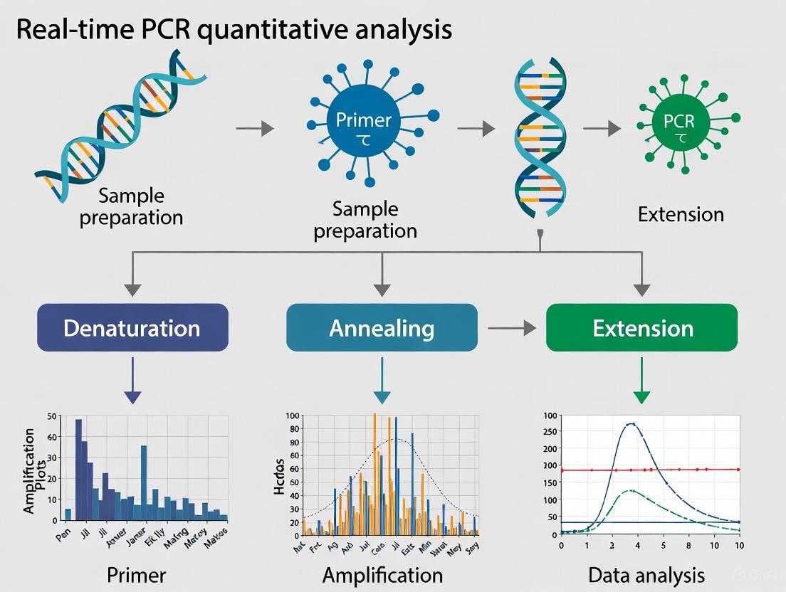
This application note delineates the fundamental operational and analytical distinctions between real-time quantitative PCR (qPCR) and end-point PCR. Framed within a comprehensive research workflow for quantitative analysis, we detail the superior quantification capabilities of qPCR, which monitors DNA amplification in real-time during the exponential phase, contrasted with the primarily qualitative nature of end-point PCR, which analyzes the final product yield. The document provides definitive protocols for both methods, supported by comparative data and workflow visualizations, to guide researchers and drug development professionals in selecting and implementing the appropriate technique for their specific molecular analyses.
The Polymerase Chain Reaction (PCR) is an in vitro enzymatic process that amplifies a specific DNA sequence from a minimal starting amount, generating thousands to millions of copies [1]. While this core principle is universal, methodological variations have given rise to distinct technologies tailored for different applications. End-point PCR, also known as conventional PCR, is a foundational method where amplification is followed by a detection step that occurs after all thermal cycles are completed, typically via agarose gel electrophoresis [2] [3]. In contrast, real-time quantitative PCR (qPCR), also referred to as real-time PCR, incorporates fluorescent chemistry to monitor the accumulation of PCR product with each cycle of amplification in real time [4] [1]. This critical difference in detection timing fundamentally transforms the data output from qualitative to quantitative, making qPCR the gold standard for applications requiring precise measurement of nucleic acid concentration, such as gene expression analysis, viral load quantification, and genotyping in drug development pipelines [1] [3].
Comparative Analysis: qPCR vs. End-Point PCR
The choice between qPCR and end-point PCR hinges on the experimental objective—whether the goal is simply to detect the presence of a sequence or to accurately determine its initial quantity. The table below summarizes the core differences, which are explored in detail in the subsequent sections.
Table 1: Core Differences Between End-Point PCR and Quantitative PCR
| Feature | End-Point PCR | Quantitative PCR (qPCR) |
|---|---|---|
| Quantification Capability | Qualitative or semi-quantitative [2] | Quantitative (absolute or relative) [2] |
| Detection Method | Agarose gel electrophoresis and staining (e.g., ethidium bromide) [2] | Fluorescent dyes (e.g., SYBR Green) or sequence-specific probes (e.g., TaqMan) [4] |
| Data Collection Point | End of all cycles (plateau phase) [5] | During every cycle (exponential phase) [5] |
| Key Quantitative Metric | Band intensity (approximate) | Threshold Cycle (Cq or Ct) [4] |
| Throughput | Lower (requires post-processing) [2] | Higher (minimal post-processing) [2] |
| Precision & Dynamic Range | Low | High [4] |
| Multiplexing Potential | Low | High (with probe-based chemistries) [4] |
| Contamination Risk | Higher (open-tube post-processing) | Lower (closed-tube system) [3] |
Fundamental Principle: Timing of Detection
The most critical distinction lies in the phase of the amplification process where data is collected.
- End-Point PCR: Analysis occurs after the reaction is complete, in the plateau phase. In this phase, reagents have been depleted, and the reaction has stopped, meaning the final amount of product does not reliably correlate with the initial template amount [5] [3]. Even samples with different starting concentrations can yield similar final product amounts, making precise quantification unreliable [3].
- Real-Time qPCR: Fluorescence is measured during the exponential phase of every cycle. In this phase, the reaction efficiency is optimal and the amount of PCR product doubles with each cycle, providing a direct and quantitative relationship between the fluorescence signal and the initial concentration of the target nucleic acid [4] [1].
The qPCR Amplification Curve and Cq Value
In qPCR, the fluorescence is plotted against cycle number to generate an amplification curve. The Cq (Quantification Cycle) value is the fractional PCR cycle number at which the fluorescent signal crosses a predefined threshold, indicating a statistically significant increase in signal over the baseline [4] [1]. There is an inverse logarithmic relationship between the Cq value and the initial target concentration: a sample with a high starting concentration will produce a detectable signal earlier, resulting in a low Cq value, while a sample with a low starting concentration will have a higher Cq value [3]. This Cq value is the cornerstone of all qPCR quantification models.
Detection Chemistries in qPCR
Real-time qPCR utilizes two primary types of fluorescent chemistries:
- DNA-Binding Dyes (e.g., SYBR Green): These dyes fluoresce brightly when bound to double-stranded DNA. They are cost-effective and convenient but will bind to any dsDNA in the reaction, including non-specific products and primer-dimers, which can lead to overestimation of the target concentration [4] [6].
- Sequence-Specific Probes (e.g., TaqMan Probes): These oligonucleotide probes are labeled with a fluorescent reporter and a quencher. The close proximity of the quencher suppresses the reporter's fluorescence until the probe is hydrolyzed by the 5' nuclease activity of the DNA polymerase during amplification. This mechanism ensures that fluorescence is generated only upon successful amplification of the specific target sequence, providing greater specificity and enabling multiplexing (detection of multiple targets in a single tube) [4] [6].
The following diagram illustrates the fundamental workflows of both techniques, highlighting the key difference: the point of detection.
Experimental Protocols
Protocol: Standard End-Point PCR
This protocol is adapted from established molecular biology guides for conventional PCR amplification [7] [8].
I. Research Reagent Solutions
Table 2: Key Reagents for End-Point PCR
| Reagent | Function | Typical 50 µL Reaction |
|---|---|---|
| Template DNA | Contains the target sequence to be amplified. | 10-500 ng [7] |
| Forward & Reverse Primers | Define the 5' and 3' ends of the target sequence. | 0.1-1 µM each [7] |
| Taq DNA Polymerase | Heat-stable enzyme that synthesizes new DNA strands. | 1.25 units [8] |
| dNTP Mix | Building blocks (dATP, dCTP, dGTP, dTTP) for new DNA strands. | 200 µM each [8] |
| PCR Buffer (with MgCl₂) | Provides optimal chemical environment; Mg²⁺ is a cofactor for the polymerase. | 1X concentration [7] |
| Sterile dH₂O | Brings the reaction to the final volume. | To volume |
II. Step-by-Step Procedure
Reaction Setup:
- Prepare a master mix on ice containing all common reagents (water, buffer, dNTPs, polymerase) to minimize pipetting errors and ensure consistency between samples.
- Aliquot the master mix into individual PCR tubes.
- Add template DNA and primers to their respective tubes. Gently mix and briefly centrifuge to collect the contents at the bottom of the tube.
- If using a thermal cycler without a heated lid, overlay the reaction with a drop of mineral oil to prevent evaporation [8].
Thermal Cycling:
- Place the tubes in a thermal cycler and run the following program [7]:
- Initial Denaturation: 94°C for 2 minutes (activates hot-start enzymes, ensures complete denaturation).
- Amplification (25-35 cycles):
- Denature: 94°C for 30 seconds.
- Anneal: 55-65°C* for 30 seconds.
- Extend: 72°C for 1 minute per kilobase of expected product.
- Final Extension: 72°C for 5-10 minutes (ensures all products are fully extended).
- Hold: 4°C indefinitely.
*The annealing temperature should be optimized, typically 5°C below the primer's melting temperature (Tm) [7].
- Place the tubes in a thermal cycler and run the following program [7]:
Post-Amplification Analysis by Gel Electrophoresis:
- Prepare a 1-2% agarose gel in TAE or TBE buffer containing a DNA intercalating dye like ethidium bromide or a safer alternative.
- Mix 2-10 µL of the PCR product with a DNA loading dye and load into the gel wells. Include a DNA molecular weight ladder.
- Run the gel at 5-10 V/cm until bands are adequately separated.
- Visualize the gel under UV light. The presence of a band at the expected size confirms amplification.
Protocol: Real-Time qPCR for Gene Expression
This protocol outlines a two-step reverse transcription qPCR (RT-qPCR) approach, which offers flexibility for analyzing multiple targets from a single RNA sample [4].
I. Research Reagent Solutions
Table 3: Key Reagents for Two-Step RT-qPCR
| Reagent (Step 1: Reverse Transcription) | Function |
|---|---|
| Total RNA or mRNA | The template for cDNA synthesis. Purity and integrity are critical. |
| Reverse Transcriptase | Enzyme that synthesizes complementary DNA (cDNA) from RNA. |
| dNTP Mix | Building blocks for the cDNA strand. |
| Primers (Random Hexamers, Oligo-dT, or Gene-Specific) | Initiate cDNA synthesis from various regions or the 3' end of mRNAs. |
| RNase Inhibitor | Protects RNA templates from degradation. |
| Reagent (Step 2: qPCR) | Function |
|---|---|
| cDNA (from Step 1) | Template for qPCR amplification. |
| qPCR Master Mix | Contains DNA polymerase, dNTPs, Mg²⁺, and optimized buffer. |
| Fluorescent Chemistry | SYBR Green dye or TaqMan probe assay for detection. |
| Forward & Reverse Primers | Define the amplicon for SYBR Green. For TaqMan, the assay includes primers and a probe. |
II. Step-by-Step Procedure
Step 1: Reverse Transcription (RNA to cDNA)
- In a nuclease-free tube on ice, combine:
- 1 pg–1 µg of total RNA
- Reverse transcription primers (e.g., 50 ng Random Hexamers or 500 ng Oligo-dT)
- 1 mM dNTPs
- Nuclease-free water to a final volume of 10-15 µL.
- Heat the mixture to 65°C for 5 minutes to denature RNA secondary structure, then immediately place on ice.
- Add the remaining components:
- 1X Reverse Transcriptase Buffer
- 20 U RNase Inhibitor
- 200 U Reverse Transcriptase
- Mix gently and incubate in a thermal cycler:
- For Random Hexamers: 25°C for 10 minutes (primer annealing), followed by 37-42°C for 30-60 minutes (cDNA synthesis).
- For Oligo-dT: 37-42°C for 30-60 minutes.
- Inactivate the enzyme by heating to 70°C for 15 minutes. The resulting cDNA can be used immediately in qPCR or stored at -20°C.
Step 2: Quantitative PCR (cDNA Amplification and Detection)
- Assay Design: Design and validate primers with high efficiency (90-110%). For SYBR Green, ensure specificity by checking for primer-dimer formation and non-specific amplification. For TaqMan, use commercially available or custom-designed assays [4].
- Reaction Setup:
- Prepare a qPCR master mix on ice containing:
- 1X qPCR Master Mix (with appropriate dye or enzyme)
- Forward and Reverse Primers (e.g., 200-400 nM each) or a pre-formulated TaqMan Assay
- Nuclease-free water
- Aliquot the master mix into a qPCR plate.
- Add a diluted volume of the cDNA from Step 1 (e.g., 1-5 µL per 20 µL reaction). Include no-template controls (NTCs) and, for relative quantification, reference gene assays.
- Seal the plate with an optical adhesive film and centrifuge briefly.
- Prepare a qPCR master mix on ice containing:
- Thermal Cycling and Data Acquisition:
- Place the plate in the real-time PCR instrument. The instrument will run a thermal cycling protocol similar to end-point PCR but will measure the fluorescence in each well at the end of each annealing or extension cycle.
- A typical fast-cycling protocol might be:
- Initial Denaturation: 95°C for 2-10 minutes.
- Amplification (40 cycles):
- Denature: 95°C for 15 seconds.
- Anneal/Extend & Acquire Data: 60°C for 30-60 seconds.
- Data Analysis:
- The instrument's software will generate an amplification plot and assign a Cq value to each reaction.
- For relative gene expression, use the Comparative Cq (ΔΔCq) method to calculate fold-change in gene expression between experimental and control groups, normalized to one or more stable reference genes [4].
Application in Drug Development and Research
The quantitative nature of qPCR makes it indispensable in the pharmaceutical and biotechnology industries. Key applications include:
- Biomarker Discovery and Validation: qPCR is used to quantify expression levels of potential mRNA or microRNA biomarkers in patient samples [4] [9].
- Pharmacogenomics: Studying how genetic variations (SNPs) affect drug response by using allelic discrimination assays [4].
- Viral Load Monitoring: Precisely quantifying viral titers (e.g., HIV, HCV) in patient serum to monitor disease progression and antiviral treatment efficacy [1] [3].
- Cell and Gene Therapy: Assessing vector copy number in transduced cells and monitoring expression of therapeutic transgenes [2].
- Toxicology Studies: Evaluating changes in gene expression profiles of drug-metabolizing enzymes or stress response genes in pre-clinical models.
Within a rigorous real-time PCR quantitative analysis workflow, the distinction between end-point PCR and qPCR is foundational. End-point PCR remains a powerful, low-cost tool for applications demanding only qualitative confirmation of a target's presence, such as cloning or genotyping. However, for any research or diagnostic question requiring accurate, sensitive, and reproducible quantification of nucleic acids—from basic gene expression studies to critical drug development assays—real-time qPCR is the unequivocal method of choice. Its ability to measure amplification during the exponential phase via Cq analysis, combined with closed-tube workflows and advanced detection chemistries, provides the data integrity necessary for robust scientific conclusions.
Within the framework of real-time PCR (qPCR) quantitative analysis workflows, a foundational decision for researchers is selecting the appropriate quantification method. The choice between absolute quantification and relative quantification is dictated by the experimental question, the required output, and the available resources [10]. Absolute quantification determines the exact amount of a target nucleic acid in a sample, expressed as a concrete number (e.g., copies per microliter). In contrast, relative quantification measures the change in target quantity relative to a reference sample, such as an untreated control, and expresses this change as a fold-difference (e.g., n-fold induction or repression) [10] [11].
This application note delineates the core principles, applications, and procedural protocols for both methods to guide researchers and drug development professionals in selecting and implementing the optimal quantification strategy for their study.
Core Concepts and Comparative Analysis
Absolute Quantification
Absolute quantification provides a direct count of target molecules. Two primary methodologies are employed:
- Standard Curve Method (qPCR): This method quantitates unknown samples by comparing them to a standard curve constructed from samples of known concentration [10]. The absolute quantities of the standards must be determined by an independent method, such as spectrophotometry (A260 measurement) [10].
- Digital PCR (dPCR) Method: A more recent innovation, dPCR partitions a sample into thousands of individual reactions. The target concentration is calculated directly from the ratio of positive to negative partitions using Poisson statistics, entirely eliminating the need for a standard curve [10] [12]. Recent studies highlight its superior accuracy for viral load quantification and rare target detection [13] [14].
Relative Quantification
Relative quantification analyzes changes in gene expression in a given sample relative to another reference sample, or calibrator (e.g., an untreated control) [10]. The result is a ratio expressing the relative change. Two common calculation methods are:
- Standard Curve Method: The quantity of the target is determined for all samples and the calibrator from a standard curve. The target quantity of each experimental sample is then divided by the target quantity of the calibrator [10].
- Comparative CT (ΔΔCT) Method: This method uses the formula 2-ΔΔCT to calculate relative expression levels. It requires that the amplification efficiencies of the target and reference gene are approximately equal and does not require a standard curve, increasing throughput [10] [11].
The following diagram illustrates the logical decision process for selecting the appropriate quantification method based on experimental goals and constraints.
Table 1: Comparative analysis of absolute and relative quantification methodologies.
| Feature | Absolute Quantification (Standard Curve) | Absolute Quantification (Digital PCR) | Relative Quantification |
|---|---|---|---|
| Core Principle | Quantitation against a standard curve of known concentrations [10] | Direct counting of molecules via sample partitioning and Poisson statistics [10] [12] | Comparison of target levels relative to a calibrator sample and a reference gene [10] |
| Primary Output | Exact quantity (e.g., copies/µL, cell equivalents) [10] | Exact quantity (e.g., copies/µL) [13] | Fold-change (n-fold difference) [10] |
| Requires Standard Curve | Yes [10] | No [10] [12] | Yes (for standard curve method) / No (for ΔΔCT method) [10] |
| Requires Reference Gene | No (but can be used for normalization) [10] | No [10] | Yes [10] [11] |
| Key Applications | Viral titer determination, copy number variation, pathogen load [10] | Rare mutation detection, liquid biopsy, absolute viral load, rare gene targets [13] [12] [14] | Gene expression studies (e.g., drug treatment, disease states) [10] [11] |
| Advantages | Established, widely accessible technology [10] | High precision, absolute quantification without standards, tolerant to inhibitors [10] [13] | Simple standardization, no need for absolute standards, high throughput for ΔΔCT [10] [15] |
| Limitations | Variability from standard curve construction and dilution errors [10] | Higher cost, lower throughput, less automated workflows [13] | Results are relative, not absolute; requires stable reference gene [10] |
Application-Specific Selection Guidelines
When to Use Absolute Quantification
- Viral Load Quantification: Determining the absolute number of viral copies in a clinical sample is critical for disease management and understanding pathogenesis [10] [13]. A 2025 study demonstrated dPCR's superior accuracy for quantifying SARS-CoV-2, influenza, and RSV compared to standard qPCR [13].
- Rare Event Detection: The high sensitivity and precision of dPCR make it ideal for detecting rare mutations in oncology (e.g., in liquid biopsies) or quantifying rare gene targets like T-Cell Receptor Excision Circles (TRECs) from limited cell samples [12] [14].
- Copy Number Variation (CNV) Analysis: Absolute determination of gene copy number per genome is a core application for both standard curve and dPCR methods [12] [11].
When to Use Relative Quantification
- Gene Expression Profiling: The vast majority of gene expression studies, such as measuring transcriptional changes in response to a drug, chemical, or disease state, are ideally suited for relative quantification [10] [11]. The result of a fold-change is biologically meaningful and sufficient.
- High-Throughput Screening: When processing hundreds of samples to compare expression levels of a defined set of genes, the comparative CT method increases throughput by eliminating the need to run a standard curve on every plate [10].
- When Absolute Standards are Unavailable: Relative quantification is the preferred method when producing a standard of known absolute concentration is difficult or impossible [15].
Experimental Protocols
Protocol 1: Absolute Quantification using a Standard Curve (qPCR)
This protocol is for absolute quantification of a DNA target using a plasmid-derived standard curve on a qPCR instrument.
Workflow Overview:
Materials:
- The Scientist's Toolkit: Key Reagents for Absolute Quantification (Standard Curve)
| Item | Function | Critical Considerations |
|---|---|---|
| Purified Standard (e.g., plasmid DNA, gDNA) | Provides known concentrations for calibration curve. | Must be a single, pure species; RNA contamination inflates copy number [10]. |
| Nucleic Acid Quantification Instrument (e.g., Spectrophotometer) | Measures concentration of standard stock (A260). | Essential for initial absolute measurement [10]. |
| qPCR Master Mix (with DNA polymerase, dNTPs) | Amplifies target sequence with fluorescence detection. | Choose dye-based (SYBR Green) or probe-based (TaqMan) chemistry [11]. |
| Target-specific Primers/Probes | Confidently amplifies and detects the target of interest. | Optimize design (amplicon 70-200 bp, Tm ~60°C, 40-60% GC) [11]. |
| Low-Binding Tubes & Pipette Tips | Used for making serial dilutions. | Prevents analyte loss due to adhesion, crucial for accuracy [10]. |
Step-by-Step Procedure:
- Standard Preparation: Prepare a high-concentration stock of purified plasmid DNA containing the target sequence. Ensure the preparation is free of RNA and contaminating DNA [10].
- Standard Quantification: Measure the concentration of the standard stock using a spectrophotometer (A260). Convert this concentration to copy number/µL using the molecular weight of the DNA [10].
- Serial Dilution: Perform a serial dilution (e.g., 10-fold) of the quantified standard over a range of at least 6 orders of magnitude (e.g., from 106 to 101 copies/µL). Prepare dilutions in a suitable buffer and divide into single-use aliquots to avoid freeze-thaw cycles [10].
- qPCR Setup: Plate the standard dilutions and unknown samples in replicates on a qPCR plate. Include a No-Template Control (NTC) to check for contamination. Use a reaction master mix containing fluorescence detection chemistry (e.g., intercalating dye or hydrolysis probe) [11] [16].
- Amplification: Run the plate on a real-time PCR instrument with the appropriate thermal cycling protocol.
- Data Analysis: The instrument software will generate a standard curve by plotting the Cq values of the standards against the log of their known concentrations. The absolute quantity of the unknown samples is determined by interpolating their Cq values from this curve [10].
Protocol 2: Absolute Quantification using Digital PCR (dPCR)
This protocol is for the absolute quantification of a DNA target without a standard curve, using a droplet-based or nanowell dPCR system.
Workflow Overview:
Materials:
- The Scientist's Toolkit: Key Reagents for Absolute Quantification (dPCR)
| Item | Function | Critical Considerations |
|---|---|---|
| dPCR Master Mix | Optimized for efficient amplification in partitioned reactions. | Formulations are often specific to the dPCR platform. |
| Target-specific Primers/Probes | Confidently amplifies and detects the target of interest. | Requires extensive optimization of concentrations for multiplex assays [13]. |
| Partitioning Device/Consumable (e.g., droplet generator, nanowell chip) | Physically divides the sample into thousands of individual reactions. | Platform-dependent (e.g., droplet vs. nanowell); defines partition volume [13] [14]. |
| dPCR Instrument (with a fluorescence reader) | Performs thermal cycling and reads fluorescence in each partition. | Systems include Bio-Rad QX200, Thermo Fisher QuantStudio Absolute, QIAGEN QIAcuity [13]. |
| Viscosity Reduction Reagents (e.g., for crude lysate) | Reduces sample viscosity for efficient partitioning. | Critical when using crude cell lysates without DNA extraction [14]. |
Step-by-Step Procedure:
- Assay Optimization: Optimize primer and probe concentrations to minimize cross-reactivity and ensure efficient amplification, especially in multiplex formats [13]. For limited samples, a crude lysate protocol bypassing DNA extraction can be validated to prevent target loss [14].
- Reaction Assembly: Assemble the PCR reaction mix containing the sample, master mix, and optimized primers/probes.
- Sample Partitioning: Load the reaction mix into the dPCR system for partitioning. This step generates thousands of nanoliter-sized droplets (ddPCR) or loads the mixture into a microfluidic chip containing fixed nanowells [13].
- Endpoint PCR Amplification: Place the partitions into a thermal cycler and run a standard PCR protocol to endpoint amplification. Real-time fluorescence monitoring within partitions (qdPCR) can be used for precise condition determination [17].
- Partition Reading and Analysis: After cycling, the instrument reads the fluorescence in each partition. Partitions are classified as positive (containing the target) or negative (not containing the target). The absolute concentration of the target in the original sample, in copies/µL, is calculated automatically by the instrument's software using Poisson statistics to account for the fact that some partitions may contain more than one molecule [10] [12].
Protocol 3: Relative Quantification using the Comparative CT(ΔΔCT) Method
This protocol is for relative quantification of gene expression using a one-step RT-qPCR approach and the 2-ΔΔCT calculation method.
Workflow Overview:
Materials:
- The Scientist's Toolkit: Key Reagents for Relative Quantification (ΔΔCT)
| Item | Function | Critical Considerations |
|---|---|---|
| RNA Integrity Number (RIN) > 8 | High-quality starting template for gene expression. | Degraded RNA skews Cq values and results. |
| One-Step RT-qPCR Master Mix | Combines reverse transcription and qPCR in a single tube. | Normalizes against variables in RNA integrity and RT efficiency [10]. |
| Target Gene Assay (Primers/Probe) | Detects the gene of interest. | Must be optimized and efficient. |
| Endogenous Control Assay (Primers/Probe) | Detects a stably expressed reference gene (e.g., GAPDH, β-actin). | Critical for normalization; expression must not vary with experimental conditions [10] [11]. |
| Calibrator Sample (e.g., Untreated Control) | Serves as the 1x sample for comparison. | All fold-change values are expressed relative to this sample [10]. |
Step-by-Step Procedure:
- Validation Experiment (Prerequisite): Before running the main experiment, perform a validation assay to demonstrate that the amplification efficiencies of the target and reference genes are approximately equal (within 10%). This is a mandatory requirement for the ΔΔCT method to be valid [10].
- RNA Preparation and Reverse Transcription: Isolate high-quality RNA from all test and calibrator samples. In a one-step RT-qPCR protocol, the reverse transcription and amplification are combined in a single well.
- RT-qPCR Setup: Plate the RNA samples in replicates. Each sample must be amplified for both the target gene of interest and the endogenous control/reference gene. A No-Template Control (NTC) should be included.
- Amplification and Cq Determination: Run the RT-qPCR protocol. The instrument will generate Cq values for the target and reference genes in every sample.
- Data Calculation:
- Calculate ΔCT for each sample: ΔCT(sample) = CT(target gene) - CT(reference gene)
- Calculate ΔΔCT: ΔΔCT = ΔCT(test sample) - ΔCT(calibrator sample). The calibrator is typically the untreated control group.
- Calculate Fold-Change: Relative Quantity (RQ) = 2-ΔΔCT [10] [11]. A value of 1 indicates no change, >1 indicates up-regulation, and <1 indicates down-regulation.
The choice between absolute and relative quantification is a critical determinant of success in any qPCR-based study. Absolute quantification, enabled by either standard curves or the emerging power of dPCR, is indispensable when an exact molecular count is the primary objective, such as in viral load monitoring or rare mutation detection. Relative quantification remains the most practical and efficient method for assessing changes in gene expression across multiple samples, as it provides biologically relevant fold-change data without the need for absolute standards.
By aligning the experimental goal with the appropriate methodology as outlined in this application note, researchers can ensure the generation of robust, reliable, and interpretable data, thereby advancing their research and drug development workflows with confidence.
Real-time quantitative polymerase chain reaction (qPCR) is a cornerstone molecular technique renowned for its sensitivity, specificity, and capacity for precise nucleic acid quantification. Its applications span critical areas of biomedical research and drug development, including gene expression analysis, viral load detection, and biomarker validation [18] [19]. The reliability of qPCR data hinges on the optimized function and integration of its core components: enzymes, primers, probes, and fluorescent reporter molecules. Adherence to established international guidelines, such as the recently updated MIQE (Minimum Information for Publication of Quantitative Real-Time PCR Experiments) guidelines, is paramount for ensuring the reproducibility, accuracy, and transparency of qPCR results [20] [21]. These guidelines provide a cohesive framework that emphasizes methodological rigor, from experimental design and execution to data analysis and reporting.
This application note provides a detailed overview of these essential qPCR components, framed within the context of a robust quantitative analysis workflow. It is structured to serve researchers, scientists, and drug development professionals by offering not only foundational knowledge but also current comparative data, detailed protocols, and validated reagent solutions to support high-quality experimental outcomes.
Core Components of Real-Time qPCR
The fundamental reaction mixture of a probe-based qPCR assay integrates several key components that work in concert to enable specific amplification and real-time detection. The core components include a DNA polymerase with 5'→3' exonuclease activity, primers to define the target amplicon, a sequence-specific probe to facilitate detection, dNTPs as the building blocks for new DNA strands, a buffer system to maintain optimal chemical conditions, and MgCl₂ as a necessary co-factor for the polymerase [19].
Fluorescent Reporter Systems
Real-time qPCR relies on fluorescent reporters whose signal intensity is directly proportional to the amount of amplified PCR product [19]. The reaction progresses through four distinct phases: the linear ground phase with background fluorescence, the early exponential phase where the signal first rises above background (defining the cycle threshold, Ct), the linear exponential phase with doubling of amplicons each cycle, and the final plateau phase where the signal ceases to increase [19]. Two primary reporter systems are employed:
- DNA-Binding Dyes (e.g., SYBR Green): These dyes bind non-specifically to double-stranded DNA, resulting in a significant (20-100 fold) increase in fluorescence upon binding [19]. Their main disadvantage is the potential to bind to non-specific products like primer-dimers, which can lead to false positive signals and overestimation of target quantity.
- Fluorescent Probes (e.g., TaqMan): Probe-based assays offer superior specificity as they require hybridization of a sequence-specific oligonucleotide to the target amplicon in addition to primer binding [19]. The most common mechanism involves the 5'→3' exonuclease activity of Taq DNA polymerase. During amplification, the polymerase cleaves a probe that is bound to the template, separating a reporter dye from a quencher dye. This separation eliminates Fluorescence Resonance Energy Transfer (FRET), resulting in a detectable fluorescent signal [19].
Table 1: Comparison of qPCR Fluorescent Reporter Systems
| Feature | DNA-Binding Dyes (SYBR Green) | Hydrolysis Probes (TaqMan) |
|---|---|---|
| Specificity | Lower - binds any dsDNA | Higher - requires specific probe hybridization |
| Cost | Lower | Higher |
| Assay Design | Simpler, requires only primers | More complex, requires primers and probe |
| Multiplexing | Not possible | Possible with different reporter dyes |
| Primary Application | Single-target detection, presence/absence | Absolute quantification, SNP genotyping, multiplex detection |
Probe Technologies and Configurations
Probe-based assays have evolved to offer enhanced performance. Key configurations include:
- Dual-Labeled Probes: Feature a reporter dye (e.g., FAM, VIC, TET) at the 5' end and a quencher dye (e.g., TAMRA, BHQ) at the 3' end. The use of dark quenchers like BHQ, which dissipate energy as heat, reduces background signal compared to fluorescent quenchers like TAMRA [19].
- Minor Groove Binder (MGB) Probes: Incorporate an MGB moiety at the 3' end, which stabilizes the probe-DNA duplex. This allows for the use of shorter probes, which is advantageous for targeting sequences with high specificity, such as in single nucleotide polymorphism (SNP) assays [19].
Applications and Comparative Performance
The specificity and quantitative nature of probe-based qPCR make it indispensable for a wide range of applications in research and diagnostics [19].
- SNP Genotyping: This method is a powerful tool for analyzing single base substitutions. It uses two allele-specific probes, each labeled with a different reporter dye (e.g., FAM and VIC). During amplification, the probe matching the perfect allele sequence binds stably and is cleaved, emitting fluorescence, while a probe with a single-base mismatch binds unstably and is not cleaved, resulting in no signal [19].
- Viral Detection and Quantification: qPCR is a gold standard for detecting and quantifying viral pathogens. For instance, during the COVID-19 pandemic, diagnostic assays targeted specific genes of SARS-CoV-2 (e.g., S, E, M, N). The presence of the virus in a sample is indicated by an increase in fluorescence signal corresponding to the amplification of these targets [13] [19].
- Gene Expression Analysis: By converting mRNA to cDNA and then performing qPCR, researchers can quantify transcript levels with high sensitivity, detecting differences even in low-abundance mRNAs [19].
- DNA Methylation Analysis: Bisulfite-treated DNA can be analyzed with probes designed to distinguish between methylated and unmethylated cytosine bases, allowing for the assessment of epigenetic modifications [19].
Comparison with Emerging Technologies
While qPCR remains a robust and widely used method, emerging technologies like digital PCR (dPCR) and next-generation sequencing (NGS) offer complementary capabilities. A 2025 study comparing dPCR and real-time RT-PCR for respiratory virus detection (Influenza A/B, RSV, SARS-CoV-2) found that dPCR demonstrated superior accuracy and precision, particularly for samples with high viral loads [13]. dPCR's absolute quantification without the need for a standard curve makes it less susceptible to inhibitors and complex sample matrices, offering potential for enhanced diagnostic accuracy [13].
Similarly, a 2025 study on Helicobacter pylori detection in pediatric biopsies compared an IVD-certified qPCR kit, a PCR-HRM method, and NGS. While all three methods showed similar detection rates, the PCR-based methods were slightly more sensitive, identifying two additional positive samples missed by NGS [22]. This highlights that NGS, though powerful for detecting multiple pathogens simultaneously and characterizing complex samples, is currently limited by cost and complexity, making PCR variants a more attractive and cost-effective option for routine targeted diagnostics [22].
Table 2: Comparison of Quantitative Nucleic Acid Detection Platforms
| Platform | Key Principle | Quantification | Throughput | Key Advantage | Key Limitation |
|---|---|---|---|---|---|
| Real-Time qPCR | Fluorescence detection during thermal cycling | Relative (requires standard curve) | High | Well-established, cost-effective, fast | Susceptible to PCR inhibitors |
| Digital PCR (dPCR) | End-point fluorescence in partitioned reactions | Absolute (no standard curve) | Medium | High precision, resistant to inhibitors | Higher cost, lower throughput |
| nCounter NanoString | Color-coded probe hybridization | Digital (direct counting) | High | No enzymatic reaction, high multiplexing | Limited dynamic range for high copy numbers |
| Next-Generation Sequencing (NGS) | Massively parallel sequencing | Digital (read counts) | Very High | Unbiased, detects novel targets | High cost, complex data analysis |
Experimental Protocols
Protocol 1: TaqMan Probe-Based qPCR for Gene Expression
Objective: To relatively quantify the expression level of a target gene in extracted RNA samples.
Workflow Overview: The following diagram illustrates the complete workflow from sample preparation to data analysis.
Materials:
- Extracted total RNA
- Reverse transcriptase kit
- TaqMan Gene Expression Assay (pre-designed primers and probe) or custom-designed primers/probe
- TaqMan Fast Advanced Master Mix (contains Taq polymerase, dNTPs, buffer, MgCl₂)
- Nuclease-free water
- 96-well or 384-well optical reaction plates
- Real-time PCR instrument
Procedure:
- RNA Quality Control: Assess RNA integrity and concentration using spectrophotometry (e.g., Nanodrop) or fluorometry (e.g., Qubit).
- Reverse Transcription: Convert 100 ng - 1 µg of total RNA to cDNA using a reverse transcriptase enzyme according to the manufacturer's protocol.
- qPCR Reaction Setup:
- Thaw and gently mix all reagents. Prepare the master mix on ice.
- For a single 20 µL reaction: 10 µL of 2X Master Mix, 1 µL of 20X TaqMan Gene Expression Assay, X µL of cDNA template (recommended equivalent of 10-100 ng input RNA), and nuclease-free water to 20 µL.
- Include a no-template control (NTC) by replacing cDNA with water.
- Pipette the reaction mix into the optical plate in triplicate for each sample.
- qPCR Run:
- Seal the plate and centrifuge briefly.
- Load the plate into the real-time PCR instrument.
- Use the following standard two-step cycling protocol:
- Hold Stage: 50°C for 2 minutes, 95°C for 20 seconds.
- PCR Stage (40 cycles): 95°C for 1 second, 60°C for 20 seconds.
- Data Analysis:
- Set the fluorescence threshold in the exponential phase of the amplification plot to determine the quantification cycle (Cq) for each reaction.
- Use the comparative Cq method (ΔΔCq) to calculate the relative fold-change in gene expression, normalizing to an endogenous reference gene and a calibrator sample [20].
Protocol 2: Multiplex qPCR for Viral Detection
Objective: To simultaneously detect and differentiate multiple viral targets (e.g., Influenza A, Influenza B, RSV) from a single respiratory sample.
Materials:
- Nasopharyngeal swab sample in viral transport media
- Automated nucleic acid extraction system (e.g., KingFisher Flex, STARlet) with appropriate kits
- Commercial multiplex respiratory panel kit (e.g., Seegene Allplex) or custom-designed multiplex assay
- Real-time PCR instrument capable of detecting multiple fluorophores
Procedure:
- Sample Preparation: Subject the respiratory sample to mechanical lysis, if necessary, to break down mucus and release viral particles [13].
- Nucleic Acid Extraction: Extract RNA using an automated platform and a viral RNA/pathogen kit. Include an internal control during extraction to monitor extraction efficiency and potential PCR inhibition [13].
- Multiplex qPCR Setup:
- The multiplex master mix will contain multiple sets of forward/reverse primers and probes, each probe labeled with a spectrally distinct fluorophore (e.g., FAM for Influenza A, VIC for Influenza B, Cy5 for RSV).
- Aliquot the master mix into the PCR plate and add the extracted RNA template.
- qPCR Run:
- Use the cycling conditions specified by the kit manufacturer, which typically include a reverse transcription step and a subsequent PCR amplification.
- Data Interpretation:
- Analyze the amplification curves in each channel to determine the presence or absence of each virus. A sample is considered positive for a specific virus if the Cq value is below a validated cut-off.
The Scientist's Toolkit: Research Reagent Solutions
A successful qPCR experiment depends on the quality and compatibility of its core reagents. The following table details essential materials and their critical functions within the workflow.
Table 3: Essential Reagents for Probe-Based qPCR Assays
| Reagent / Kit | Function / Description | Example Products / Notes |
|---|---|---|
| Nucleic Acid Extraction Kit | Isolates high-purity DNA/RNA from complex biological samples; critical for removing PCR inhibitors. | MagMax Viral/Pathogen Kit, STARMag Universal Cartridge Kit [13] |
| Reverse Transcriptase Kit | Synthesizes complementary DNA (cDNA) from an RNA template for gene expression studies. | High-Capacity cDNA Reverse Transcription Kit |
| Taq DNA Polymerase | Thermostable enzyme that amplifies DNA; for probe-based assays, must possess 5'→3' exonuclease activity. | AmpliTaq Gold, FastStart Taq DNA Polymerase |
| qPCR Master Mix | Optimized buffer containing Taq polymerase, dNTPs, MgCl₂, and stabilizers for robust amplification. | TaqMan Fast Advanced Master Mix |
| Sequence-Specific Primers | Short oligonucleotides that define the start and end of the target amplicon for amplification. | Custom-designed, HPLC-purified; critical for specificity. |
| Hydrolysis Probe (TaqMan) | Sequence-specific oligonucleotide with reporter and quencher dyes; enables real-time detection via 5' nuclease assay. | Dual-labeled probes, MGB probes [19] |
| Commercial Assay Panels | Pre-validated, multiplexed assays for detecting multiple targets simultaneously. | Allplex Respiratory Panel, TaqMan Array Cards |
| Internal Positive Control | Control for nucleic acid extraction and amplification; detects PCR inhibition in clinical samples. | RNAse P gene detection in human samples [19] |
The integrity of real-time PCR quantitative analysis is fundamentally dependent on the careful selection and application of its core components. From the design of specific primers and probes to the choice of a robust enzyme system, each element must be optimized to ensure data accuracy and reproducibility. As the field advances, adherence to the MIQE 2.0 guidelines provides a critical framework for standardizing practices and reporting, thereby enhancing the reliability of research outcomes [20]. Furthermore, understanding the relative strengths and limitations of qPCR in comparison to emerging technologies like dPCR and NGS empowers scientists to select the most appropriate platform for their specific research or diagnostic question. By leveraging the detailed protocols, comparative data, and reagent solutions outlined in this application note, researchers and drug development professionals can confidently execute qPCR experiments that yield precise, reproducible, and biologically meaningful results.
Real-time PCR, also known as quantitative PCR (qPCR), is a powerful molecular technique that combines polymerase chain reaction amplification with fluorescent detection to monitor the accumulation of DNA products in real time [9]. Unlike conventional PCR that provides endpoint analysis, qPCR allows researchers to quantify the initial amount of a specific nucleic acid target with remarkable precision and over a wide dynamic range [11]. The fundamental output of a qPCR reaction is the amplification curve, a graphical representation of fluorescence signal versus PCR cycle number that contains critical information about the reaction performance and enables reliable quantification [23].
The amplification curve is typically divided into three distinct phases: the baseline phase with no detectable fluorescence increase, the exponential phase where product doubling occurs with each cycle, and the plateau phase where reaction components become depleted and amplification ceases [24]. Understanding the characteristics and proper interpretation of each phase, particularly the exponential phase, is essential for accurate gene quantification, proper assay validation, and meaningful experimental conclusions in both research and diagnostic applications [25] [26].
Core Principles of the Amplification Curve
The Three Phases of PCR Amplification
Baseline Phase: During the initial PCR cycles (typically cycles 1-15), the fluorescent signal remains at background levels as the accumulated product has not yet reached the detection threshold of the instrument. The baseline represents the background fluorescence that must be corrected for accurate quantification [27] [23].
Exponential Phase: This is the most critical phase for quantification, characterized by a rapid increase in fluorescence where the amount of PCR product theoretically doubles with each cycle. During this phase, all reaction components (primers, dNTPs, enzyme) are in excess, fueling consistent amplification efficiency. The exponential phase appears as a straight line when fluorescence is plotted on a logarithmic scale against cycle number [25] [24].
Plateau Phase: In the final phase of amplification, the reaction slows and eventually stops as essential components become depleted (primers, dNTPs) or the DNA polymerase loses activity. The fluorescence signal reaches a maximum level and shows minimal increase with additional cycles. Data from this phase are not considered quantitative [25] [24].
Understanding the Threshold Cycle (Ct)
The Threshold Cycle (Ct), also known as quantification cycle (Cq), is a fundamental parameter in qPCR analysis defined as the PCR cycle number at which the amplification curve crosses the fluorescence threshold [23]. This threshold is set within the exponential phase of amplification where the reaction is most efficient and reproducible. The Ct value is inversely proportional to the starting quantity of the target nucleic acid—a lower Ct value indicates a higher initial amount of target template, while a higher Ct value indicates a lower initial amount [23].
Proper threshold setting is crucial for accurate Ct determination. The threshold should be set:
- Sufficiently above the background fluorescence to avoid premature threshold crossing
- Within the exponential phase of all amplification curves being compared
- At a position where amplification curves display parallel log-linear phases [27]
Figure 1: The three phases of a qPCR amplification curve and determination of the Ct value. The Ct is identified where the curve crosses the threshold during the exponential phase.
The Critical Role of PCR Efficiency
PCR efficiency refers to the rate at which the target sequence is amplified during each cycle of the PCR reaction [26]. Ideally, efficiency should be 100%, meaning the target DNA doubles with every cycle during the exponential phase. In practice, efficiency is expressed as a percentage or a decimal value (e.g., 100% = 1.0, 90% = 0.9) and is a critical parameter that directly impacts quantification accuracy [24].
Efficiency can be calculated from a standard curve generated using serial dilutions of a known template concentration. The formula for calculating efficiency is:
E = 10(-1/slope) - 1
Where the slope is derived from the plot of Ct values against the logarithm of the template concentration [26] [28]. For a perfect reaction with 100% efficiency, the slope should be -3.32 [28].
Table 1: Interpretation of PCR Efficiency Values
| Efficiency Value | Slope | Interpretation | Impact on Quantification |
|---|---|---|---|
| 100% (2.0) | -3.32 | Ideal efficiency | Accurate quantification |
| 90-110% | -3.1 to -3.6 | Acceptable range | Minimal error |
| <90% | >-3.6 | Low efficiency | Underestimation of quantity |
| >110% | <-3.1 | Apparent super-efficiency | Overestimation of quantity |
Experimental Protocols
Protocol 1: Determining Amplification Efficiency
Objective: To determine the PCR amplification efficiency for a specific assay using a serial dilution series.
Materials Required:
- Template DNA or cDNA of known concentration
- qPCR master mix
- Target-specific primers and/or probes
- Nuclease-free water
- Appropriate qPCR instrument and consumables
Procedure:
- Prepare a 5- or 10-fold serial dilution series of the template spanning at least 5 orders of magnitude (e.g., 1:10, 1:100, 1:1,000, 1:10,000, 1:100,000).
- For each dilution, prepare qPCR reactions in triplicate according to the following setup:
- 10 µL qPCR master mix (2X concentration)
- 2 µL forward primer (10 µM)
- 2 µL reverse primer (10 µM)
- 1 µL probe (5 µM) if using hydrolysis probes
- 5 µL template DNA from appropriate dilution
- Adjust total volume to 20 µL with nuclease-free water
- Include no-template controls (NTC) containing nuclease-free water instead of template.
- Run the qPCR reaction using the following cycling conditions:
- Initial denaturation: 95°C for 2-10 minutes
- 40 cycles of:
- Denaturation: 95°C for 15 seconds
- Annealing/Extension: 60°C for 1 minute
- After the run, record the Ct values for each dilution.
Data Analysis:
- Plot the mean Ct value for each dilution against the logarithm of the template concentration or dilution factor.
- Generate a linear regression trendline through the data points.
- Calculate the slope of the trendline.
- Calculate the amplification efficiency using the formula: E = 10(-1/slope) - 1
- Assess the linearity of the standard curve using the coefficient of determination (R²). A value of R² ≥ 0.98 indicates excellent linearity [28].
Protocol 2: Validating Assay Performance Using MIQE Guidelines
Objective: To comprehensively evaluate qPCR assay performance according to MIQE (Minimum Information for Publication of Quantitative Real-Time PCR Experiments) guidelines.
Materials Required:
- Test samples with varying target concentrations
- Reference gene assay with confirmed performance
- qPCR reagents as in Protocol 1
- Melt curve analysis capability (for SYBR Green assays)
Procedure:
- Specificity Assessment:
- For hydrolysis probe assays: Verify single amplification curves with characteristic sigmoidal shape.
- For SYBR Green assays: Perform melt curve analysis post-amplification by gradually increasing temperature from 60°C to 95°C while monitoring fluorescence. A single peak indicates specific amplification.
- Analyze no-template controls for absence of amplification.
Sensitivity and Dynamic Range Determination:
- Follow Protocol 1 to establish the linear dynamic range.
- Determine the limit of detection (LOD) as the lowest concentration at which 95% of positive samples are detected [28].
Precision Evaluation:
- Run intra-assay replicates (same run) and inter-assay replicates (different runs) for samples with high, medium, and low target concentrations.
- Calculate the coefficient of variation (CV) for Ct values. CV should be <5% for technical replicates [25].
Efficiency Confirmation:
- Confirm that assay efficiency falls within 90-110% as calculated in Protocol 1.
Table 2: Quality Control Criteria for qPCR Assay Validation
| Parameter | Acceptance Criterion | Quality Assessment Method |
|---|---|---|
| Amplification Efficiency | 90-110% | Standard curve from serial dilutions |
| Dynamic Range | 5-6 orders of magnitude | Linear regression of dilution series |
| Specificity | Single peak in melt curve | Melt curve analysis (SYBR Green) |
| Precision | CV < 5% for Ct values | Replicate analysis |
| Linearity | R² ≥ 0.98 | Coefficient of determination |
| No-Template Control | No amplification or Ct > 40 | Include NTC in each run |
Protocol 3: Relative Quantification Using the ΔΔCt Method
Objective: To determine relative changes in gene expression between different experimental conditions.
Materials Required:
- cDNA samples from test and control conditions
- Validated assays for target gene and reference gene(s)
- qPCR reagents as in previous protocols
Procedure:
- For each sample (test and control), run qPCR reactions for both the target gene and reference gene(s) in triplicate.
- Include appropriate controls (NTC, positive control).
- Record Ct values for all reactions.
Data Analysis:
- Calculate the ΔCt for each sample: ΔCt = Ct(target gene) - Ct(reference gene)
- Calculate the ΔΔCt: ΔΔCt = ΔCt(test sample) - ΔCt(control sample)
- Calculate the relative quantification (RQ) or fold change: RQ = 2-ΔΔCt
Important Considerations:
- The ΔΔCt method assumes the amplification efficiencies of the target and reference genes are approximately equal and close to 100% [26].
- If efficiencies are not equal, use an efficiency-corrected calculation: RQ = (Etarget)^(-ΔCttarget) / (Ereference)^(-ΔCtreference) [27]
- Select reference genes that show stable expression across experimental conditions.
Data Analysis and Interpretation
Troubleshooting Amplification Curve Abnormalities
Table 3: Common Amplification Curve Abnormalities and Solutions
| Abnormality | Possible Causes | Solutions |
|---|---|---|
| Irregular or jagged curves | Instrument instability, bubbles in reaction | Centrifuge plates before run; check instrument calibration [25] |
| Late Ct values (>35) | Low template concentration, inhibition | Increase template amount; purify sample [29] |
| No amplification | Template degradation, primer design issues | Check RNA/DNA quality; redesign primers |
| Multiple peaks in melt curve | Non-specific amplification, primer dimers | Optimize annealing temperature; redesign primers |
| Efficiency >110% | PCR inhibition in concentrated samples, pipetting errors | Dilute samples; improve pipetting technique [29] |
| Efficiency <90% | Poor primer design, reaction inhibitors | Redesign primers; purify template |
The Scientist's Toolkit: Essential Reagents and Materials
Table 4: Essential Research Reagent Solutions for qPCR
| Reagent/Material | Function | Considerations |
|---|---|---|
| qPCR Master Mix | Provides DNA polymerase, dNTPs, buffer, and salts | Choose based on application; may include passive reference dye [25] |
| Hydrolysis Probes (TaqMan) | Target-specific detection with fluorophore and quencher | Provides high specificity; requires custom design [11] |
| SYBR Green Dye | Intercalating dye that binds double-stranded DNA | Cost-effective; requires melt curve analysis for specificity [11] |
| Passive Reference Dye (ROX) | Normalizes for non-PCR related fluorescence fluctuations | Included in many master mixes; essential for plate-to-plate normalization [25] |
| Primers | Sequence-specific oligonucleotides for target amplification | Design for 15-30 bp length, 40-60% GC content, Tm ~60-65°C [11] |
| Nuclease-Free Water | Solvent for reactions | Prevents RNA/DNA degradation |
| dNTPs | Nucleotides for DNA synthesis | Component of master mix |
| UNG Enzyme | Prevents carryover contamination | Degrades uracil-containing DNA from previous reactions [9] |
Advanced Concepts and Applications
The Impact of Efficiency on Quantification Accuracy
PCR efficiency significantly impacts quantification accuracy, particularly in relative gene expression studies using the ΔΔCt method. Even small deviations from 100% efficiency can introduce substantial errors in calculated fold-changes [26].
The error introduced by efficiency discrepancies can be calculated as: Error (%) = [(2^n/(1+E)^n) × 100)] - 100 Where E = efficiency of PCR and n = cycle number [26].
For example, if the PCR efficiency is 0.9 instead of 1.0 at a threshold cycle of 25, the resulting error will be 261%, meaning the calculated expression level would be 3.6-fold less than the actual value [26].
Figure 2: Comprehensive qPCR workflow highlighting the critical role of amplification efficiency throughout the experimental process. The cyclic nature demonstrates that unacceptable efficiency requires returning to assay optimization.
High-Throughput Data Analysis Methods
For laboratories processing large numbers of samples, high-throughput analysis methods such as the "dots in boxes" approach can efficiently visualize multiple assay characteristics simultaneously [28]. This method plots PCR efficiency on the y-axis against ΔCq (difference between Cq of NTC and lowest template dilution) on the x-axis, creating a graphical box where successful experiments should fall (efficiency 90-110%, ΔCq ≥3) [28].
Each data point can be assigned a quality score (1-5) based on multiple parameters including linearity, reproducibility, fluorescence consistency, curve steepness, and shape. This approach allows rapid evaluation of overall experimental success across multiple targets and conditions [28].
The qPCR amplification curve contains a wealth of information that, when properly demystified, enables robust and reliable nucleic acid quantification. Understanding the three distinct phases of amplification—baseline, exponential, and plateau—provides the foundation for accurate data interpretation. The exponential phase is particularly critical as it provides the Ct values used for quantification and reflects the PCR efficiency that fundamentally impacts calculation accuracy.
Proper experimental design, including rigorous assay validation according to MIQE guidelines, careful attention to efficiency determination, and appropriate implementation of quantification methods (ΔΔCt or standard curve), ensures generation of biologically meaningful results. Troubleshooting common amplification curve abnormalities and understanding their underlying causes further strengthens experimental outcomes.
As qPCR continues to be a cornerstone technique in molecular biology, clinical diagnostics, and drug development, mastery of amplification curve interpretation remains an essential skill for researchers seeking to generate quantitative data that withstands scientific scrutiny.
Within the framework of real-time PCR quantitative analysis research, the initial phases of RNA extraction and cDNA synthesis constitute the foundational pillars determining the entire workflow's success. This application note details a standardized, robust protocol designed to overcome common challenges such as RNA degradation, genomic DNA contamination, and inhibitor carryover, which are critical for generating reliable, reproducible gene expression data in drug development and clinical research settings [30] [31]. The procedures outlined herein are optimized to ensure high nucleic acid integrity and reverse transcription fidelity, directly impacting the accuracy of downstream quantitative PCR (qPCR) results.
Technical Specifications and Performance Data
Selecting appropriate reagents based on performance metrics is crucial for a robust workflow. The following tables summarize key quantitative data from comparative evaluations of different RNA extraction methods and reverse transcriptase enzymes.
Table 1: Comparison of RNA Extraction Methods from Challenging Samples
| Extraction Method / Kit | Sample Type | Average Yield | Purity (A260/A280) | Key Advantages |
|---|---|---|---|---|
| FastPure Cell/Tissue Kit (Vazyme) [30] | Rat liver, HEK 293 cells | High | High | Good integrity, high yield, and high purity |
| Modified SDS-Based Method [32] | Musa spp. (banana) tissues | 2.92-6.30 µg/100 mg | 1.83-2.25 | Effective for polysaccharide/polyphenol-rich tissues |
| Stool RNA Purification Kit (Norgen) [31] | Human stool | High | High | High purity, sensitive downstream detection |
| TRIzol Reagent [33] [32] | Various tissues | Variable | Variable | Effective lysis; may require additional purification |
Table 2: Reverse Transcriptase Enzyme Performance Characteristics
| Enzyme Type | Reaction Temperature | Reaction Time | RNase H Activity | Ideal For |
|---|---|---|---|---|
| AMV Reverse Transcriptase [34] | 42°C | 60 min | High | Standard templates |
| MMLV Reverse Transcriptase [34] | 37°C | 60 min | Medium | Longer transcripts (<7 kb) |
| Engineered MMLV (e.g., SuperScript IV) [34] | 50-55°C | 10 min | Low | Challenging RNA, high GC content |
| HiScript IV (Vazyme) [30] | 37-50°C | 5-15 min | No | Low-input/degraded RNA, fast workflow |
Optimized Protocol for RNA Extraction
Sample Lysis and Homogenization
The first critical step is the effective disruption of cells or tissues while maintaining RNA integrity.
- Animal Tissues/Cells: For manual extraction from tissues like rat liver or cultured cells like HEK 293, use ~10 mg of tissue or 1x10^6 cells. Homogenize in lysis buffer containing guanidine salts using bead beating or mechanical homogenization. For Vazyme's FastPure Kit, homogenization is followed by centrifugation to clear the lysate [30].
- Plant Tissues: For challenging plant samples like Musa spp., grind 100 mg of tissue in liquid nitrogen. Use a modified SDS-based lysis buffer supplemented with PVP and β-mercaptoethanol to bind polyphenols and prevent oxidation [32].
- Complex Samples (e.g., Stool): Homogenize 200 µL of sample preserved in RNAlater in a bead tube with the kit's lysis buffer at 2,850 rpm for 5 minutes [31].
RNA Purification and DNase Treatment
Purification removes contaminants like proteins, salts, and most critically, genomic DNA.
- Silica-Membrane Purification: This is the basis for many kit-based methods (e.g., Vazyme, Norgen, Qiagen). The cleared lysate is mixed with ethanol and loaded onto a silica membrane. RNA binds while contaminants pass through [30] [31].
- DNase I Treatment: To eliminate gDNA contamination, apply an RNase-free DNase I solution directly onto the silica membrane and incubate at room temperature for 15 minutes [31] [33]. This step is essential for accurate gene expression analysis.
- Alternative gDNA Removal: As an alternative to DNase I, thermolabile double-strand-specific DNases (e.g., ezDNase) can be used. They are inactivated by a short 5-minute heating step at 55°C, simplifying the workflow and reducing RNA loss [34].
- Washing and Elution: Wash the membrane with an ethanol-based wash buffer to remove salts and other residues. Elute the pure RNA in nuclease-free water [33]. Elution at room temperature can improve yield [35].
RNA Quality Assessment
Rigorous quality control is non-negotiable for reliable downstream results.
- Quantification and Purity: Use a spectrophotometer (e.g., NanoDrop) to measure concentration. Assess purity via A260/A280 ratio (ideal range: 1.8-2.1) and A260/A230 ratio (ideal >2.0), indicating minimal protein/phenol or salt/organic solvent contamination, respectively [36] [31] [32].
- Integrity Assessment: Evaluate RNA integrity by agarose gel electrophoresis. Sharp, clear ribosomal RNA bands (28S and 18S in eukaryotes) with the 28S band approximately twice the intensity of the 18S band indicate intact RNA [30] [32]. For a more precise measure, use an RNA Integrity Number (RIN) or Qubit RNA IQ Assay [32].
Optimized Protocol for cDNA Synthesis
Reaction Setup and Primer Selection
The reverse transcription reaction must be carefully assembled based on the RNA template and research goals.
- RNA Input: Use 10 pg to 1 µg of total RNA per 20 µL reaction, with 500 ng being a standard starting point for gene expression studies. Normalize RNA input across samples for accurate comparative analysis [36].
- Primer Choice: Selection depends on the application:
- Oligo(dT) Primers: Anneal to the 3' poly-A tail of mRNA, ideal for synthesizing cDNA for reverse transcriptase qPCR (RT-qPCR) of protein-coding genes. They provide specific priming but can lead to 5' bias in long transcripts [34].
- Random Hexamers: Prime throughout the RNA sequence, ideal for degraded RNA, non-polyadenylated RNAs, or when analyzing multiple regions of a transcript [36] [34].
- Gene-Specific Primers: Provide the most specific priming but are only suitable for synthesizing cDNA for one target.
- Blended Primers: Some kits (e.g., Bio-Rad iScript) use a blend of oligo(dT) and random hexamers to provide comprehensive coverage [36].
Table 3: The Scientist's Toolkit: Essential Reagents for RNA to cDNA Workflow
| Item | Function | Example Products & Notes |
|---|---|---|
| Lysis Buffer | Disrupts cells, inactivates RNases | Often contains guanidine thiocyanate (commercial kits) or SDS (for plants) [30] [32]. |
| Silica Spin Column | Binds and purifies RNA | Found in most commercial kits; enables efficient washing [30] [31]. |
| DNase I, RNase-free | Digests contaminating genomic DNA | Critical for accurate RT-qPCR. Can be used on-column or in-solution [31] [34]. |
| Reverse Transcriptase | Synthesizes cDNA from RNA template | Engineered enzymes (e.g., SuperScript IV, HiScript IV) offer high stability and yield [30] [34]. |
| dNTP Mix | Building blocks for cDNA synthesis | Use high-quality dNTPs at 0.5-1 mM each [34]. |
| RNase Inhibitor | Protects RNA template from degradation | Essential for handling low-abundance targets [34]. |
Thermal Cycling and Post-Synthesis Handling
The incubation conditions are key to efficient cDNA synthesis, especially for complex RNA templates.
- Primer Annealing: Incubate the reaction mix at 25°C for 5-10 minutes to allow primers to anneal to the RNA template [36] [34].
- cDNA Synthesis (Polymerization): Incubate at the optimal temperature for the reverse transcriptase. For thermostable enzymes like SuperScript IV or HiScript IV, use 50-55°C for 10-20 minutes. The higher temperature helps denature RNA secondary structures, leading to more full-length cDNA and higher yields [30] [34].
- Reaction Termination: Inactivate the enzyme by heating at 85°C for 5 minutes or 95°C for 1 minute [36] [34].
- cDNA Storage: For immediate use, store diluted cDNA at 4°C. For long-term storage, prepare aliquots and store at -20°C or -80°C to minimize freeze-thaw cycles, which can degrade cDNA [36].
Workflow and Evaluation Diagrams
The following diagram illustrates the complete integrated workflow from sample to cDNA, highlighting key decision points and quality control checkpoints.
The protocol's effectiveness is demonstrated through a comparative evaluation of different methods, as illustrated below.
This application note provides a detailed, evidence-based framework for establishing a robust and reliable workflow from RNA extraction to cDNA synthesis. By adhering to the optimized protocols and quality control measures outlined—including the selection of appropriate extraction methods for specific sample types, the use of engineered reverse transcriptases for high-efficiency cDNA synthesis, and rigorous quality assessment—researchers can significantly enhance the accuracy and reproducibility of their real-time PCR quantitative data. The successful application of this workflow is confirmed by its validation in downstream quantitative real-time PCR (qRT-PCR), enabling precise gene expression analysis crucial for advancing research in drug development and molecular diagnostics [30] [32].
Executing a Reliable qPCR Assay: A Step-by-Step Protocol from Primer Design to Data Acquisition
In the realm of molecular biology and drug development, the real-time quantitative PCR (qPCR) workflow stands as a cornerstone technology for gene expression analysis, validation of therapeutic targets, and diagnostic assay development. The reliability of any qPCR experiment is fundamentally dependent on the initial primer design phase, where strategic decisions determine the specificity, efficiency, and accuracy of subsequent quantitative results. Poorly designed primers can lead to costly experimental failures, false positives in diagnostic applications, and irreproducible data in research settings. This application note establishes a comprehensive protocol for designing PCR primers with an emphasis on two critical aspects: ensuring target specificity through bioinformatic tools like Primer-BLAST and proactively avoiding single nucleotide polymorphisms (SNPs) that could compromise assay performance. By integrating these considerations into a standardized workflow, researchers and drug development professionals can achieve superior experimental outcomes with enhanced reliability and reduced optimization time.
Foundational Principles of PCR Primer Design
Effective primer design extends beyond merely identifying complementary sequences flanking a target region. It requires careful balancing of multiple physicochemical properties that collectively determine primer behavior during amplification. The following parameters represent the essential foundation upon which specific and robust PCR assays are built:
Table 1: Essential Parameters for Optimal Primer Design
| Parameter | Optimal Range | Rationale & Impact |
|---|---|---|
| Primer Length | 18–30 bases [37] [38] | Balances specificity and binding efficiency; shorter primers may cause nonspecific binding. |
| Melting Temperature (Tm) | 60–64°C [38]; Optimal difference between paired primers: ≤ 2°C [38] | Ensures simultaneous binding of both primers to the template. |
| GC Content | 40–60% [37]; Ideal: 50% [38] | Provides sequence complexity while maintaining appropriate Tm; extremes can hinder binding. |
| GC Clamp | Presence of 2 G or C bases within the last 5 bases at the 3' end [37] | Stabilizes primer-template binding at the critical elongation point. |
| 3' End Stability | ΔG > -9 kcal/mol for secondary structures [38] | Prefers stable 3' ends to reduce false priming while avoiding overly stable dimers. |
Several critical design elements must be avoided to prevent assay failure. Repetitive sequences, including runs of four or more identical bases (e.g., AAAA) or dinucleotide repeats (e.g., ATATAT), can cause mispriming [37]. Similarly, primers must be screened for self-complementarity and cross-complementarity between forward and reverse primers, which can lead to primer-dimer formation that consumes reaction resources and reduces target amplification efficiency [37] [39]. The ΔG value for any potential secondary structures should be weaker (more positive) than -9.0 kcal/mol [38].
Advanced Strategy: Ensuring Specificity and Avoiding SNP Interference
The Critical Importance of Specificity Checking
Primer specificity ensures that amplification originates exclusively from the intended genetic target, a non-negotiable requirement for both basic research and clinical diagnostic applications. Non-specific amplification can generate false positive signals, quantitate irrelevant targets, and completely invalidate experimental results. This risk is particularly acute in genetically complex samples or when detecting low-abundance transcripts. The Primer-BLAST tool, developed and maintained by the National Center for Biotechnology Information (NCBI), provides an integrated solution that combines primer design with automated specificity validation against comprehensive nucleotide databases [40] [41].
The Critical Importance of SNP Avoidance
Single nucleotide polymorphisms represent the most common form of genetic variation in genomes. When undetected SNPs occur within primer binding sites, particularly at the critical 3' end, they can severely impede primer annealing and extension, leading to allele dropout, reduced amplification efficiency, and genotyping inaccuracies [42]. This failure mode has profound implications for clinical diagnostics where heterozygous samples might be misclassified, or for pathogen detection where variant strains could escape identification. Proactive SNP checking during primer design is significantly more effective than post-hoc troubleshooting of failed assays.
Integrated Workflow for Specificity and SNP Avoidance
Diagram: Primer Design and Validation Workflow
Protocol: Designing SNP-Aware Primers Using Primer-BLAST
This step-by-step protocol ensures the production of specific, SNP-resistant primers suitable for sensitive qPCR applications in drug development and clinical research.
Pre-Design Sequence Analysis
- Sequence Acquisition: Obtain the complete mRNA reference sequence (RefSeq) for your target gene, preferably using the NCBI Nucleotide database. The accession number format (e.g., NM_XXXXXX) is ideal for subsequent steps [40].
- Flanking Sequence Determination: For the genomic region of interest, ensure you have at least 50 nucleotides of high-quality sequence information both upstream and downstream of your target site [42]. This provides adequate context for robust primer design.
- SNP Screening: Before designing primers, use the dbSNP database (maintained by NCBI) to identify known polymorphisms within your target region. Manually inspect the primer binding regions, especially the final 5 nucleotides at the 3' end, and exclude any candidates where polymorphisms occur at these critical positions.
Primer-BLAST Specificity Analysis
- Access the Tool: Navigate to the NCBI Primer-BLAST submission form [40] [41].
- Input Template: Enter the RefSeq accession number or FASTA sequence in the "PCR Template" section. Using an mRNA reference sequence ensures the tool can design primers specific to particular splice variants [40].
- Configure Primer Parameters:
- Set Specificity Checking Parameters (Critical Step):
- Under "Primer Pair Specificity Checking Parameters," select the appropriate source organism [40] [41]. This restricts the search and increases precision.
- Choose the "Refseq mRNA" database for most gene expression applications [43]. For broader coverage, "Refseq representative genomes" or "core_nt" are alternatives [41].
- Enable the option "Primer must span an exon-exon junction" when working with RNA/cDNA to prevent amplification of genomic DNA contaminants [41] [43]. Set the requirement for annealing to both exons at the junction.
- Execute and Analyze: Click "Get Primers" to submit. Primer-BLAST will return only primer pairs that are computationally predicted to be specific to your intended target [41]. Carefully review the output to confirm the primer binding locations and verify the in silico specificity.
Post-Design Validation
- Secondary Structure Analysis: Use tools such as the IDT OligoAnalyzer or the UNAFold Tool to check all selected primer pairs for self-dimers, cross-dimers, and hairpin structures [38]. Confirm that the ΔG values for any potential secondary structures are more positive than -9.0 kcal/mol [38].
- Experimental Validation: Always validate primer performance empirically using a dilution series to calculate amplification efficiency (target: 90–110%) [4]. Include melt curve analysis for SYBR Green-based assays to confirm a single, specific amplification product.
Advanced Applications and Reagent Solutions
For particularly challenging applications involving highly multiplexed PCR or superior SNP discrimination, specialized technologies and reagent systems have been developed.
Table 2: Research Reagent Solutions for Advanced Primer Applications
| Technology / Reagent | Primary Function | Key Application Context |
|---|---|---|
| Self-Avoiding Molecular Recognition Systems (SAMRS) [39] | Nucleobase analogs that pair with natural bases but not with other SAMRS, reducing primer-dimer formation. | Highly multiplexed PCR; superior SNP discrimination in complex backgrounds. |
| PACE (PCR Allele Competitive Extension) [42] | Advanced allele-specific PCR chemistry for SNP and Indel detection using competitive primer extension. | High-throughput genotyping in agricultural, aquaculture, and clinical research; diagnostic assay development. |
| SADDLE Algorithm [44] | Computational algorithm for designing highly multiplexed PCR primer sets that minimize primer dimer formation. | Large NGS panels; multiplexed qPCR assays targeting dozens to hundreds of targets simultaneously. |
| Double-Quenched Probes [38] | qPCR probes with internal quenchers (ZEN/TAO) that lower background fluorescence and increase signal-to-noise. | Sensitive quantitative gene expression analysis; pathogen detection with improved quantification accuracy. |
Mastering primer design with rigorous attention to specificity and SNP avoidance is not merely a technical exercise but a fundamental requirement for generating reliable, reproducible qPCR data. The integrated workflow presented herein—combining foundational design principles with the computational power of Primer-BLAST and proactive SNP screening—provides researchers and drug development professionals with a robust framework for assay development. This systematic approach significantly de-risks the experimental process, reduces costly reagent waste, and accelerates the translation of research findings into actionable results. By adopting these protocols, laboratories can enhance the quality of their genetic analysis workflows, ultimately supporting the development of more precise therapeutic interventions and diagnostic tools.
Quantitative real-time polymerase chain reaction (qPCR) is a cornerstone technique in molecular biology for sensitive, specific, and reproducible quantification of gene expression. However, its accuracy is significantly influenced by variables such as RNA integrity, cDNA synthesis efficiency, pipetting inaccuracies, and presence of PCR inhibitors [45]. To control for this technical variation, normalization using stably expressed reference genes (often housekeeping genes) is essential [45]. The selection of inappropriate reference genes, whose expression varies under experimental conditions, is a common source of erroneous conclusions in gene expression studies. It has been demonstrated that the expression of typical housekeeping genes can vary significantly across different tissues, developmental stages, and experimental treatments [46] [47]. This article provides a comprehensive guide to the selection and validation of stable reference genes, introducing the geNorm algorithm and other critical tools within the context of a robust qPCR workflow.
Several algorithms have been developed to statistically evaluate the expression stability of candidate reference genes. Using multiple tools in tandem is considered best practice, as it provides a more robust validation than any single method [48].
Table 1: Key Algorithms for Reference Gene Validation
| Algorithm | Underlying Principle | Key Output | Special Feature |
|---|---|---|---|
| geNorm | Pairwise comparison of expression ratios between candidate genes [49]. | Stability measure (M); lower M value indicates greater stability. Also determines the optimal number of reference genes (V) [49] [46]. | Identifies the best pair of genes rather than a single gene. |
| NormFinder | Models expression variation within and between sample groups [50]. | Stability value; considers both intragroup and intergroup variation [51] [52]. | Less sensitive to co-regulation of genes compared to geNorm. |
| BestKeeper | Based on the pairwise correlation analysis of Ct values [52]. | Standard deviation (SD) and coefficient of variance (CV); genes with SD > 1 are considered unstable [53]. | Works well with a high number of candidates and sample types. |
| RefFinder | A web-based comprehensive tool that integrates the results from geNorm, NormFinder, BestKeeper, and the comparative ΔCt method [51] [48]. | A comprehensive ranking index. | Provides an overall stability ranking by combining multiple algorithms. |
The geNorm Algorithm: A Closer Look
The geNorm algorithm, introduced by Vandesompele et al. in 2002, has become one of the most widely used methods for reference gene validation, with over 22,000 scientific citations [49]. Its core principle is a pairwise comparison. For each pair of candidate genes, it calculates the pairwise variation ( V ) as the standard deviation of the logarithmically transformed expression ratios. A stability measure (M) is then defined for each gene as the average pairwise variation of that gene with all other tested candidate genes. Genes are stepwise eliminated, with the least stable gene (highest M value) removed at each step, until the two most stable genes remain [49].
A critical feature of geNorm is its ability to determine the optimal number of reference genes required for accurate normalization. This is done by calculating a normalization factor (NF) based on the geometric mean of the best performing genes. The pairwise variation ( Vn/V{n+1} ) between sequential normalization factors (e.g., NF(n) and NF({n+1})) is calculated. A default cutoff of ( V < 0.15 ) is suggested, below which the inclusion of an additional reference gene is not required [49] [48].
Originally implemented as a Microsoft Excel tool, the modern version of geNorm is now integrated into qbase+ software (available from CellCarta following its acquisition of Biogazelle), which offers enhanced features, including handling of missing data and availability for multiple operating systems [49]. Free and open-source implementations are also available in R (NormqPCR), Python (eleven, rna-genorm), and via web interfaces [49].
Practical Applications and Case Studies
The condition-specific nature of reference gene stability is illustrated by numerous studies across diverse organisms. The following examples demonstrate that there is no universal reference gene and validation is always required.
Table 2: Example Stable Reference Genes from Various Studies
| Organism | Experimental Condition | Identified Stable Reference Genes | Citation |
|---|---|---|---|
| Floccularia luteovirens (fungus) | Salt stress | ACT, EF-Tu | [51] |
| Drought stress | γ-TUB, UBC-E2 | [51] | |
| Heat stress | EF-Tu, γ-TUB | [51] | |
| Across all samples | H3, SAMDC | [51] | |
| Lentinula edodes (fungus) | High-temperature stress | TUB, UBI | [53] |
| Nelumbo nucifera (lotus) | Various tissues & development | TBP, UBQ, EF-1α, GAPDH (condition-dependent) | [46] |
| Mythimna loreyi (insect) | Developmental stages, tissues | RPL27, RPL10 | [47] |
| Temperature treatments | AK, RPL10 | [47] | |
| Barnyard millet (plant) | Drought stress | UBC5, α-TUB | [48] |
| Salinity stress | GAPDH | [48] | |
| Heat stress | EF-1α, RP II | [48] |
Case Study: Validation in an Insect Model
A 2024 study on the insect Mythimna loreyi provides a robust example of the validation workflow. Researchers evaluated 13 candidate reference genes under various biotic and abiotic conditions, including different developmental stages, tissues, and temperature treatments [47]. The expression stability was analyzed using the ΔCt method, BestKeeper, NormFinder, GeNorm, and the comprehensive platform RefFinder. The results were highly condition-specific. For instance, RPL27 and RPL10 were the most stable for developmental stages and tissues, while AK and RPL10 were best for temperature treatments, and EF and RPS3 were optimal for analyzing mating status [47]. This underscores the necessity of validating reference genes for each unique experimental setup.
A Step-by-Step Experimental Protocol for Validation
This protocol outlines the key steps for selecting and validating reference genes for qPCR normalization.
Candidate Gene Selection and Primer Design
- Select Candidates: Choose 8-12 candidate genes from literature, genomic databases, or transcriptome data. Ideal candidates are involved in basic cellular maintenance (e.g., cytoskeleton, protein degradation, transcription). Include genes from different functional pathways to avoid co-regulation [51] [47] [48].
- Design Primers: Design primers with the following criteria using tools like Primer-BLAST:
- Amplicon length: 70-200 bp.
- Primer melting temperature (Tm): 58-62°C.
- Exon-exon junction spanning to avoid genomic DNA amplification.
- Validate Primer Specificity: Perform standard PCR and analyze products on an agarose gel to confirm a single amplicon of the expected size. Verify reaction specificity further with a melt curve analysis after qPCR, which should yield a single peak [48].
RNA Extraction, cDNA Synthesis, and qPCR
- Sample Preparation: Collect samples encompassing all experimental conditions, tissues, and time points to be studied. Use at least three biological replicates per condition. Flash-freeze in liquid nitrogen and store at -80°C [54] [53].
- RNA Extraction: Isolate total RNA using a reliable kit or method. Treat samples with DNase I to remove genomic DNA contamination. Assess RNA integrity by agarose gel electrophoresis (clear ribosomal RNA bands) and determine purity using a spectrophotometer (A260/A280 ratio ~2.0) [54] [46].
- cDNA Synthesis: Synthesize cDNA from equal amounts of total RNA (e.g., 1 µg) using a reverse transcription kit with random hexamers and/or oligo-dT primers. Dilute the synthesized cDNA to a consistent concentration for qPCR [53] [46].
- qPCR Run: Perform qPCR reactions in technical duplicates or triplicates. Use a reaction mix containing SYBR Green dye. The standard thermal cycling conditions are: initial denaturation (95°C for 2-5 min), followed by 40 cycles of denaturation (95°C for 15 s), annealing (primer-specific Tm, e.g., 60°C for 15 s), and extension (72°C for 20 s). Include a no-template control (NTC) for each primer pair [52] [48].
Data Analysis and Validation
- Calculate Amplification Efficiency: Generate a standard curve using a serial dilution of cDNA (e.g., 1:5, 1:25, 1:125). Plot the log of the dilution factor against the Ct value. The slope of the line is used to calculate the amplification efficiency (E) using the formula: ( E = (10^{-1/slope} - 1) \times 100\% ). Primers with an efficiency between 90% and 110% are typically acceptable [52] [48].
- Evaluate Stability: Input the Ct values for all candidate genes and samples into the stability analysis tools: geNorm, NormFinder, BestKeeper, and RefFinder.
- Determine the Optimal Number of Genes: Use the geNorm output for the pairwise variation (V) to decide how many reference genes are needed. If ( V_{n/n+1} < 0.15 ), 'n' genes are sufficient [48].
- Experimental Validation: Confirm the suitability of the selected genes by using them to normalize a target gene with a known expression pattern. For example, a stress-responsive gene like HSP90 [51] or SOD1 [48] can be analyzed. The normalized expression profile should align with expected biological behavior, confirming the reliability of the chosen reference genes.
The Scientist's Toolkit
Table 3: Essential Research Reagents and Solutions
| Reagent / Solution | Function / Application | Example Notes |
|---|---|---|
| Total RNA Isolation Kit | Extraction of high-quality, intact RNA from biological samples. | Kits specifically designed for tissues rich in polysaccharides/polyphenols (e.g., plants, fungi) are available [54] [46]. |
| DNase I, RNase-free | Removal of contaminating genomic DNA from RNA preparations to prevent false positives. | A critical step; often included in modern RT kits or performed separately [46]. |
| Reverse Transcription Kit | Synthesis of complementary DNA (cDNA) from an RNA template. | Kits often include a mix of random hexamers and oligo-dT primers for comprehensive cDNA representation [53]. |
| SYBR Green qPCR Master Mix | Provides all components (enzyme, dNTPs, buffer, dye) for efficient and specific qPCR amplification. | Enables real-time detection of amplified DNA via binding to double-stranded DNA [45] [53]. |
| TaqMan Assays | Sequence-specific probes for target detection, offering higher specificity than intercalating dyes. | Ideal for multiplexing or when high specificity is paramount [50]. |
The following diagram illustrates the complete workflow for reference gene selection and validation.
Within the broader context of real-time PCR quantitative analysis workflow research, the reproducibility and accuracy of results are fundamentally dependent on the meticulous optimization of the reaction itself. The qPCR workflow is a multi-faceted process where the performance of each component—from reagent formulation to instrument programming—directly impacts the final quantitative data [9]. This application note provides detailed protocols for optimizing key stages of the qPCR reaction, specifically the master mix, thermocycling conditions, and experimental plate setup, to ensure data integrity for researchers, scientists, and drug development professionals.
Optimizing the qPCR Master Mix
The master mix is the core biochemical environment of the qPCR reaction. Its composition dictates the efficiency, specificity, and sensitivity of the amplification. Optimization is critical for overcoming challenging templates and achieving robust, reproducible results.
Core Components and Their Optimization
A qPCR master mix contains several key components, each requiring careful consideration. The table below summarizes the optimization strategies for these core reagents.
Table 1: Optimization Guidelines for qPCR Master Mix Components
| Component | Typical Concentration | Optimization Consideration | Effect of Sub-optimal Concentration |
|---|---|---|---|
| Magnesium (Mg²⁺) | 1.5 - 2.0 mM [55] | Concentration depends on template, buffer, and dNTPs, all of which can chelate Mg²⁺. | Too low: No PCR product. Too high: Non-specific amplification and spurious products [55]. |
| Primers | 0.1 - 0.5 µM each [55] | Ideal length is 20-30 nt with 40-60% GC content. Primer pairs should have melting temperatures (Tm) within 5°C of each other [11] [55]. | Higher concentrations can promote secondary priming and dimer formation, leading to non-specific amplification [55]. |
| dNTPs | 200 µM of each [55] | Lower concentrations (50-100 µM) can enhance fidelity but reduce yield. | Higher concentrations can increase yield but may reduce polymerization fidelity [55]. |
| DNA Polymerase | 1.25 - 1.5 units per 50 µL reaction [55] | Enzyme choice is critical. Standard Taq is common; hot-start polymerases increase specificity; proofreading enzymes (e.g., Pfu) enhance fidelity [55]. | Insufficient enzyme leads to low yield; too much can increase background signal or non-specific products. |
| Template DNA | 1 pg – 1 ng (plasmid); 1 ng – 1 µg (genomic) [55] | High-quality, purified template is essential. Higher concentrations can decrease specificity in high-cycle reactions. | Impure or degraded template is a primary cause of PCR failure. High concentration can cause non-specific binding. |
Detection Chemistry Selection
The choice of detection chemistry is a primary decision in assay design, balancing specificity, cost, and complexity.
- DNA Intercalating Dyes (e.g., SYBR Green I): These dyes bind non-specifically to double-stranded DNA, offering versatility and cost-effectiveness [56] [11]. However, they will bind to any dsDNA, including primer-dimers and non-specific products, which can lead to overestimation of the target concentration [11].
- Hydrolysis Probes (e.g., TaqMan): These are target-specific oligonucleotides with a 5' fluorescent reporter and a 3' quencher [56]. The DNA polymerase's 5' exonuclease activity cleaves the probe during amplification, separating the reporter from the quencher and generating a fluorescent signal [56] [11]. This method offers high specificity but requires custom design and is more costly [11].
- Other Probe-Based chemistries, such as Molecular Beacons and Locked Nucleic Acid (LNA) probes, offer alternative strategies for enhancing specificity and stability, though they may require more extensive design and optimization [11].
Optimizing Thermocycling Conditions
The thermocycling protocol drives the amplification reaction. Precise control of temperature and time at each stage is vital for efficient and specific product formation.
Key Cycling Parameters
A standard qPCR run involves an initial denaturation followed by 35-40 cycles of three core steps, with fluorescence measurement typically occurring at the end of the annealing/extension phase [11].
Table 2: Key Parameters for qPCR Thermocycling Optimization
| Step | Typical Temperature | Typical Duration | Optimization Guidelines |
|---|---|---|---|
| Initial Denaturation | 95°C | 2 - 10 min | Time depends on the DNA polymerase's heat-activated mechanism [56] [55]. |
| Denaturation | 95°C | 10 - 30 sec | Sufficient to fully melt dsDNA. Longer times may be needed for templates with high GC content [56] [55]. |
| Annealing | 5°C below the lowest primer Tm (often 50-60°C) [55] | 15 - 30 sec [55] | The most critical parameter to optimize. Use a gradient PCR to determine the ideal temperature for specific primer binding [55]. If spurious products are observed, test higher temperatures [55]. |
| Extension | 68 - 72°C [56] [11] | 1 min per 1 kb [55] | For products < 1 kb, 45-60 seconds is often sufficient. For probe-based chemistries, annealing and extension are often combined at 60°C [56]. |
Figure 1: A generalized workflow for a qPCR thermocycling protocol, highlighting the repetitive nature of the amplification cycles where fluorescence is measured.
Experimental Design and Plate Setup
A well-designed plate layout is fundamental for generating statistically sound data and is a key aspect of the MIQE guidelines [57]. Systematic planning minimizes errors and facilitates efficient data analysis.
Essential Information and Controls
Every well on a qPCR plate must be defined by three minimal pieces of information: sample_id (unique nucleic acid sample), target_id (primer set/probe), and prep_type (type of nucleic acid preparation) [57]. Including appropriate controls is non-negotiable for validating results.
- No Template Control (NTC): Contains all master mix components except the template DNA/RNA. Any amplification indicates contamination [11].
- No Reverse Transcriptase Control (-RT): For RT-qPCR, this control lacks the reverse transcriptase enzyme. Amplification indicates genomic DNA contamination [57].
- Positive Control: Contains a known template for the target. A lack of amplification suggests an assay error [11].
- Endogenous Control: A consistently expressed housekeeping gene used for normalization in relative quantification [11].
Systematic Plate Planning
A robust strategy is to design a small, logical rectangle that represents one full technical replicate of the experiment, then duplicate this rectangle across the plate [57]. This approach is interpretable by both people and analysis software and simplifies loading with multichannel pipettes.
The following diagram illustrates the logical process for designing a qPCR plate experiment, from defining the biological question to creating a physical plate layout.
Figure 2: The logical workflow for designing a qPCR plate experiment, emphasizing systematic planning from hypothesis to physical layout.
Protocol: Setting Up a 48-Well Plate Plan
This protocol outlines the setup for an experiment measuring 4 genes across 3 biological replicates with both +RT and -RT preparations, totaling 48 wells [57].
Define Variables:
target_id_levels: ACT1, BFG2, CDC19, DED1sample_id_levels: rep1, rep2, rep3prep_type_levels: +RT, -RT
Create a Row Key: Assign targets to rows.
Create a Column Key: Assign samples and preparation types to columns. This requires 6 columns (3 biological replicates × 2 prep types).
Generate the Plate Plan: Combine the row and column keys using a blank plate template.
This creates a systematic layout where, for example, row A contains ACT1 for all samples, and columns 1 & 2 contain rep1 for +RT and -RT, respectively, across all targets.
Data Analysis and Quantification
The fundamental output of qPCR is the amplification plot, which tracks fluorescence versus cycle number. The Threshold Cycle (Ct) is the cycle number at which the fluorescent signal crosses a threshold set within the exponential phase of amplification [56] [11]. A sample with a high starting template concentration will have a low Ct, while a low concentration will have a high Ct.
Figure 3: A core data analysis workflow for qPCR, from the raw amplification plot to final quantification using either absolute or relative methods.
Quantification is typically achieved through one of two methods:
- Absolute Quantification: Determines the exact copy number of the target in the sample by comparing Ct values to a standard curve of known concentrations [9] [11].
- Relative Quantification: Determines the change in target quantity relative to a control sample (e.g., untreated), using the ΔΔCt method [11]. This method normalizes the Ct of the target gene to an endogenous reference gene (
ΔCt = Ct_target - Ct_reference) and then compares this value to the calibrator sample (ΔΔCt = ΔCt_treated - ΔCt_control). The fold-change is calculated as 2^(-ΔΔCt) [11].
The Scientist's Toolkit: Research Reagent Solutions
Table 3: Essential Reagents and Kits for qPCR Workflows
| Item | Function/Description |
|---|---|
| Hot-Start DNA Polymerase | Increases assay specificity by preventing enzyme activity until the first high-temperature denaturation step, reducing primer-dimer formation and non-specific amplification [55]. |
| qPCR Master Mix | A pre-mixed solution containing buffer, dNTPs, polymerase, and MgCl₂. Available formulated for different detection chemistries (e.g., SYBR Green or TaqMan probes) to provide consistency and save setup time [55]. |
| Reverse Transcriptase Kit | For RT-qPCR, these kits convert RNA to cDNA. Systems are available for one-step (combined RT and qPCR) or two-step (separate reactions) protocols [9] [56]. |
| DNA/RNA Extraction Kit | Provides high-quality, purified nucleic acid templates, which is a critical first step for successful qPCR. Example: QIAamp DNA Mini Kit [58] [59]. |
| Primers & Probes | Oligonucleotides designed for specific target amplification and detection. Adherence to design rules (length, Tm, GC content) is crucial [11] [55]. |
| Digital PCR (dPCR) Systems | While not qPCR, dPCR is a related technology that provides absolute quantification without a standard curve by using partitioning. It can offer superior sensitivity and precision for detecting low-abundance targets, as demonstrated in pathogen detection studies [59]. |
In real-time quantitative PCR (qPCR) and reverse transcription qPCR (RT-qPCR), the extreme sensitivity that enables detection of minute amounts of nucleic acid also renders these techniques highly vulnerable to contamination and amplification artifacts. Within a rigorous qPCR workflow, controls are not merely optional but fundamental to data integrity. The Non-Template Control (NTC) and the No Reverse Transcriptase Control (No-RT) serve as critical sentinels, detecting contamination and ensuring that reported results accurately reflect the target nucleic acid. Their proper implementation and interpretation are essential for generating scientifically valid and reproducible data, particularly in drug development and diagnostic applications where false positives or negatives can have significant consequences [60] [61].
This application note details the theoretical basis, practical implementation, and troubleshooting protocols for these essential controls, providing a framework for their integration into a robust qPCR workflow.
Theoretical Foundations and Purpose of Controls
The Role of the Non-Template Control (NTC)
The NTC is a reaction mixture containing all components except the nucleic acid template. This includes master mix, primers, probes, and water [62]. Its primary function is to detect contamination or the formation of primer-dimers.
- Contamination Detection: Amplification in the NTC indicates that one or more reagent components are contaminated with template DNA, most commonly from amplicon carryover from previous PCRs, contaminated reagents, or environmental contamination [63] [61].
- Primer-Dimer Identification: In SYBR Green-based qPCR, primer-dimers can form and be amplified, generating a background signal. The NTC is crucial for identifying this non-specific amplification, which typically produces a dissociation curve peak distinct from the specific amplicon [63].
The Role of the No Reverse Transcriptase Control (No-RT)
The No-RT control is specific to RT-qPCR workflows, where the goal is to detect and quantify RNA targets. This control contains all components of the RT reaction, including the RNA sample, but lacks the reverse transcriptase enzyme [62] [64].
- Genomic DNA Contamination Detection: The most critical function of the No-RT control is to reveal the presence of contaminating genomic DNA (gDNA) in an RNA sample. Since the reverse transcription step is blocked, any amplification signal observed in the No-RT control must originate from DNA, not the RNA target [64] [65].
- Assay Specificity Verification: A well-designed RT-qPCR assay should be specific for cDNA. Amplification in the No-RT control suggests that the assay is co-amplifying gDNA, which can lead to overestimation of the true RNA expression levels [66].
The following workflow diagram outlines the logical process of incorporating these controls and interpreting their results.
Experimental Protocols and Implementation
Protocol for No-Template Control (NTC) Setup
The NTC should be included in every qPCR run, regardless of whether it is a DNA or RNA target being quantified.
Materials:
- Master mix (containing polymerase, dNTPs, buffer, salts)
- Primer/Probe set
- Nuclease-free water
- Template DNA/cDNA (omitted in NTC)
Procedure:
- Prepare Master Mix: Combine all reaction components except the template in a single tube to minimize pipetting error and cross-contamination [63].
- Aliquot Master Mix: Dispense the appropriate volume of master mix into the NTC reaction well.
- Add Water: To the NTC well, add a volume of nuclease-free water equivalent to the volume of template added to sample wells.
- Run qPCR: Execute the thermal cycling protocol alongside experimental samples.
- Data Analysis:
- Expected Result: No amplification curve (Cq value is undetermined or >40-45 cycles) [61].
- Problematic Result: An amplification curve with a Cq value <40-45. Proceed to troubleshooting (Section 4.0).
Protocol for No Reverse Transcriptase Control (No-RT) Setup
The No-RT control is essential for any RT-qPCR experiment aiming to quantify gene expression or detect RNA viruses.
Materials:
- RNA sample
- Master mix (for one-step RT-qPCR) or PCR master mix (for two-step RT-qPCR)
- Primer/Probe set
- Nuclease-free water
- Reverse Transcriptase enzyme (omitted in No-RT)
Procedure:
- Prepare Two Master Mixes: For a two-step RT-qPCR, prepare the RT reaction master mix with and without the reverse transcriptase enzyme. For a one-step RT-qPCR, prepare the master mix and split it, adding enzyme to the sample portion and omitting it from the No-RT control.
- Combine with RNA: Add the same volume of the RNA sample to both the "+RT" and the "-RT" (No-RT) reaction mixes.
- Perform Reverse Transcription: For two-step protocols, carry out the RT step. The No-RT sample should be incubated under identical conditions.
- Proceed to qPCR: Amplify both the "+RT" and "No-RT" samples using the same qPCR conditions.
- Data Analysis:
- Expected Result: The No-RT control should show a significantly higher Cq (e.g., ≥5 cycles later) than the corresponding +RT sample, or no amplification at all [66] [65]. This indicates minimal gDNA contribution.
- Problematic Result: A Cq value in the No-RT control that is similar to or only slightly higher than the +RT sample. Proceed to troubleshooting (Section 4.0).
Research Reagent Solutions
The following table details key reagents and materials essential for implementing these controls effectively.
Table 1: Essential Research Reagents for qPCR Controls
| Item | Function/Description | Application Notes |
|---|---|---|
| Nuclease-free Water | Solvent for master mixes and controls; must be free of contaminating nucleases and nucleic acids. | Critical for NTC preparation. Contaminated water is a common source of false positives in NTCs [63]. |
| UDG/UNG Enzyme | Enzyme incorporated into master mixes to prevent amplicon carryover contamination. | Degrades PCR products from previous reactions containing dUTP, reducing false positives in NTCs [63] [61]. |
| DNase I, RNase-free | Enzyme for digesting contaminating genomic DNA in RNA samples prior to RT. | Pre-treatment step to mitigate gDNA contamination, reducing signal in No-RT controls [64] [67]. |
| SYBR Green Master Mix | Intercalating dye for detecting double-stranded DNA amplification. | Enables melt curve analysis to distinguish specific product from primer-dimer in NTCs [63]. |
| Validated Primer/Probe Sets | Assays designed for specificity and validated for efficiency. | Primers should be designed to span exon-exon junctions where possible to increase gDNA insensitivity [64] [66]. |
Data Interpretation and Troubleshooting
A systematic approach to interpreting control results is vital. The following table summarizes expected results, common anomalies, and their solutions.
Table 2: Troubleshooting Guide for NTC and No-RT Controls
| Control | Expected Result | Problematic Result | Potential Cause | Corrective Action |
|---|---|---|---|---|
| Non-Template Control (NTC) | No amplification (Cq undetermined) [61]. | Amplification with low Cq. | Reagent contamination with template DNA [63] [61]. | Prepare fresh reagents from new stocks; use dedicated pre-PCR workspace; use UDG treatment [63]. |
| Amplification with high Cq (>35), low signal. | Primer-dimer formation (SYBR Green) [63] [65]. | Optimize primer concentrations; improve primer design; check melt curve for low-Tm peak [63]. | ||
| No-RT Control | No amplification or Cq significantly higher (e.g., ΔCq ≥5) than +RT sample [66]. | Cq similar to +RT sample. | Significant genomic DNA contamination in RNA sample [64] [65]. | DNase treat RNA sample; redesign primers to span an exon-exon junction [64] [67]. |
| Amplification, but NTC is clean. | Confirms gDNA contamination is sample-specific, not reagent-derived. | Use a robust DNase digestion protocol during RNA purification [67]. |
Advanced Methodologies for gDNA Contamination
For targets where gDNA contamination is persistent, or for highly repetitive sequences, advanced methods beyond simple DNase treatment and primer design can be employed.
- The ValidPrime Assay: This method uses a separate qPCR assay targeting a non-transcribed genomic region to precisely quantify the amount of gDNA present in each RT(+) sample. This gDNA-derived signal can then be computationally subtracted from the total signal, providing a more accurate measure of the RNA-derived signal without the need for a separate No-RT control for every sample/assay combination [66].
- Modified Primer Strategy: A novel approach involves using a reverse transcription primer that contains strategically placed mismatches (e.g., 4 alternating base alterations) at its 3' end. This creates a cDNA product that is slightly different from the gDNA. The subsequent qPCR primer is designed to perfectly match this modified cDNA, ensuring specific amplification of the cDNA and not the gDNA, thereby eliminating the gDNA background without physical DNA removal [67].
The integration of these controls and troubleshooting workflows into the standard qPCR procedure is summarized below.
The Non-Template Control and No-RT Control are non-negotiable components of a rigorous real-time PCR quantitative analysis workflow. Their consistent and correct application serves as the foundation for data integrity, allowing researchers to distinguish true signal from artifact. By adhering to the protocols outlined herein—meticulous reagent handling, proper workspace segregation, thoughtful assay design, and systematic troubleshooting—scientists and drug development professionals can ensure their qPCR data is reliable, reproducible, and worthy of confidence in high-stakes research and development environments.
Within the framework of real-time PCR (qPCR) quantitative analysis, the accurate determination of the quantification cycle (Cq) and the reaction efficiency is a critical foundational step. These two parameters are the bedrock upon which reliable and reproducible quantification of nucleic acids is built, directly impacting the interpretation of gene expression, pathogen load, and other molecular analyses in research and drug development [24] [68]. The Cq value represents the cycle number at which the amplification fluorescence crosses a defined threshold, indicating a point where amplification is first detectable above background [4]. Reaction efficiency (E), ideally at 100% (or a value of 2), describes the fold-increase of amplicon per cycle during the exponential phase [24]. Deviations from ideal efficiency, whether higher or lower, can lead to significant inaccuracies in calculated target quantities, with even an efficiency of 80% introducing an 8.2-fold error at a Cq of 20 compared to 100% efficiency [24]. This application note details standardized protocols for the precise determination of Cq and efficiency, ensuring data integrity throughout the qPCR workflow.
Theoretical Background and Key Concepts
The Quantification Cycle (Cq) and PCR Kinetics
The fundamental kinetics of qPCR are described by the equation: N_C = N_0 × E^Cq, where N_C is the number of amplicons at the Cq cycle, N_0 is the initial number of target molecules, and E is the amplification efficiency [68]. The Cq value is inversely proportional to the logarithm of the initial target quantity; a difference of one Cq between samples represents an E-fold difference in starting material [24]. Accurate Cq determination is therefore paramount and depends on proper baseline correction and threshold setting.
The baseline fluorescence, which is amplification-independent, must be correctly subtracted from the raw fluorescence data. Modern qPCR instruments typically fit a trendline through the fluorescence values of the early ground phase cycles and subtract this from the entire amplification curve [68]. The quantification threshold (Fq) should be set within the exponential phase of amplification, which is best identified when the amplification curve is plotted on a logarithmic (log) scale [24] [68]. It is crucial to understand that different threshold levels will yield different Cq values for the same reaction [68].
PCR Efficiency and Its Implications
PCR efficiency is defined as the ratio of target molecules at the end of a cycle to the number at the start of that cycle [24]. An efficiency of 100% (E=2) means the amplicon doubles every cycle. Efficiencies between 90% and 110% are generally considered acceptable [29]. Assays with efficiencies below 90% suffer from reduced sensitivity and dynamic range, while reported efficiencies significantly above 100% are often artifacts caused by the presence of PCR inhibitors in more concentrated samples, which flatten the standard curve slope [29]. The consistent use of efficiency-corrected calculations is essential for accurate quantification, as assuming 100% efficiency for a sub-optimal assay introduces substantial bias [68].
Experimental Protocols
Protocol 1: Determining Amplification Efficiency via Standard Curve
This method is the most common for assessing assay-specific amplification efficiency.
Materials:
- Template: Target DNA or cDNA of known high concentration.
- qPCR Reagents: Master mix, forward and reverse primers, nuclease-free water.
- Equipment: Real-time PCR instrument, calibrated pipettes.
Procedure:
- Serially Dilute Template: Prepare a minimum 5-point, 10-fold serial dilution of the template DNA, spanning a concentration range relevant to your samples. A 7-point, 10-fold series is ideal for a robust curve [24].
- Run qPCR: Amplify each dilution in replicate (at least triplicate) under your standard cycling conditions.
- Generate Standard Curve: Plot the mean Cq value for each dilution against the logarithm of its known initial concentration. The instrument software or other analysis tools will generate a line of best fit.
- Calculate Efficiency: Determine the slope of the standard curve and calculate efficiency (E) using the formula:
E = 10^(-1/slope)[24] [29]. - Interpret Results:
- A slope of -3.32 corresponds to 100% efficiency.
- A slope steeper than -3.32 (e.g., -3.5) indicates lower efficiency.
- A slope shallower than -3.32 (e.g., -3.2) suggests an artifact causing reported efficiency to exceed 100% [24].
Troubleshooting:
- Low Efficiency: Re-optimize primer concentrations, check primer design for secondary structures, or ensure reaction conditions are optimal.
- Efficiency >110%: Suspect PCR inhibition. Purify the template DNA, dilute the sample, or use an inhibitor-tolerant master mix. Re-run the standard curve, excluding the most concentrated points if they show signs of inhibition [29].
Protocol 2: Visual Assessment of Efficiency
This qualitative method is a rapid check for assays expected to have 100% efficiency, such as pre-validated TaqMan assays.
Procedure:
- Obtain Amplification Plots: Run samples and controls with your test assay.
- Set Log Scale: View the amplification plots with the fluorescence axis set to a logarithmic scale.
- Assess Parallelism: Examine the exponential phase of the amplification curves. All curves for a given assay, and ideally between different assays known to be 100% efficient, should be parallel [24].
- Interpretation: Curves that are not parallel indicate less than 100% efficiency and potential issues with the assay (See Figure 3) [24].
Table 1: Comparison of Methods for Determining PCR Efficiency
| Method | Principle | Key Steps | Quantitative Output? | Key Advantages | Key Limitations |
|---|---|---|---|---|---|
| Standard Curve | Relationship between Cq and template concentration | Serial dilution, qPCR, linear regression | Yes | Provides a numerical efficiency value; robust. | Prone to errors from imprecise pipetting and dilution [24]. |
| Visual Assessment | Parallelism of exponential-phase slopes | Plot amplification curves on a log scale | No | Quick; does not require a dilution series; not impacted by pipetting errors [24]. | Does not yield a numerical value; requires an assay with known 100% efficiency for comparison. |
Workflow for Accurate Cq and Efficiency Determination
The following diagram illustrates the integrated workflow for obtaining reliable Cq values and reaction efficiency.
The Scientist's Toolkit: Key Research Reagent Solutions
The following table outlines essential materials and reagents for executing the protocols described in this note.
Table 2: Essential Reagents and Materials for qPCR Efficiency Analysis
| Item | Function/Description | Example Applications/Notes |
|---|---|---|
| High-Fidelity DNA Polymerase | Enzyme with proofreading activity for high-quality amplicon generation and standard preparation. | Preparation of template for standard curves; reduces mutation introduction [69]. |
| qPCR Master Mix | Optimized buffer containing thermostable polymerase, dNTPs, MgCl₂, and fluorescent dye (e.g., SYBR Green) or probe. | Provides consistent reaction conditions. Choose inhibitor-tolerant formulations if sample purity is a concern [29]. |
| Validated Primer/Probe Assays | Assays designed for specific, efficient amplification. | Pre-designed TaqMan assays are guaranteed to have 100% efficiency; custom assays should be designed using specialized software [24]. |
| Nuclease-Free Water | Solvent for preparing reagents and dilutions. | Ensures reactions are not contaminated by RNases or DNases. |
| Certified Nuclease-Free Tubes and Plates | Reaction vessels that prevent sample degradation and adsorption. | Critical for maintaining template integrity and ensuring accurate pipetting during serial dilution. |
| Calibrated Pipettes | Precision instruments for accurate liquid handling. | Essential for creating accurate serial dilutions for standard curves; miscalibration is a common source of error [24]. |
Accurate determination of Cq values and reaction efficiencies is not merely a preliminary step but a fundamental component of the qPCR quantitative analysis workflow. By rigorously applying the protocols for baseline correction, threshold setting, and efficiency assessment outlined in this document, researchers and drug development professionals can ensure their data is both accurate and reliable. Adherence to these standardized methodologies, coupled with the use of high-quality reagents, forms the basis for robust gene expression analysis, pathogen quantification, and other critical applications in molecular biology.
Troubleshooting and Fine-Tuning Your qPCR Assay for Peak Performance
In real-time quantitative PCR (qPCR) workflows, the accuracy of quantitative analysis is fundamentally dependent on the specificity and efficiency of the amplification process. Primer-derived artifacts, notably primer-dimer formation and secondary structures, constitute major sources of error that skew quantification results by competing for reaction components and generating non-specific fluorescence signals [70] [71]. Primer-dimers are short, unintended amplification products that form when primers anneal to each other via complementary regions rather than to the target template [71]. Similarly, secondary structures within primers or templates can hinder proper annealing and extension. Within the context of a comprehensive qPCR workflow, systematic primer evaluation and optimization is not merely a preliminary step but a critical ongoing process that ensures data reliability, especially in drug development where quantitative accuracy directly impacts experimental conclusions and downstream decisions.
Principles of Primer Design and Pitfalls
Effective primer design establishes the foundation for successful qPCR, while poor design introduces artifacts that compromise data integrity.
Core Design Parameters
Optimal primers typically range from 20-30 nucleotides in length with an ideal GC content between 40-60%, ensuring balanced melting temperature (Tm) [72] [70]. The calculated Tm for both forward and reverse primers should fall within 58-65°C and be within 1-5°C of each other to promote simultaneous binding [72] [70] [73]. Spacing GC residues evenly throughout the primer sequence prevents stable local secondary structures. The 3' ends are particularly critical; they should not contain more than two G or C bases in the last five nucleotides (a phenomenon known as a "GC clamp") to minimize mispriming [70]. Furthermore, runs of three or more identical nucleotides, especially G or C, should be avoided as they promote misalignment [70].
Mechanisms of Artifact Formation
Primer-dimerization occurs through two primary mechanisms: self-dimerization, where a single primer contains self-complementary regions, and cross-dimerization, where forward and reverse primers have complementary sequences [71]. These interactions create free 3' ends that DNA polymerase can extend, generating short, spurious amplification products. Secondary structures like hairpins occur when a primer folds back on itself, forming stable intra-molecular bonds that prevent the primer from binding to its intended template [73]. These structures are thermodynamically favored at lower temperatures, explaining why they often form during the assay's annealing phase.
Experimental Protocols for Evaluation and Optimization
This section provides detailed methodologies for diagnosing and resolving primer-related issues.
Protocol 1: In silico Primer Analysis
- Objective: To computationally predict potential dimerization and secondary structures prior to synthesis.
- Materials: Primer sequences in text format, computer with internet access, primer analysis software (e.g., Primer3, OligoAnalyzer Tool).
- Methodology:
- Sequence Input: Enter the forward and reverse primer sequences separately into the analysis tool.
- Self-Complementarity Check: Use the software to analyze each primer for hairpin formation and self-dimerization. Pay close attention to stability (ΔG) predictions; more negative values indicate stronger, more problematic structures.
- Cross-Dimerization Check: Input both forward and reverse primers to assess potential inter-primer interactions.
- Specificity Verification: Perform a BLAST (Basic Local Alignment Search Tool) analysis against the appropriate genome database (e.g., NCBI) to ensure primers are unique to the target sequence and do not bind to non-target sites, especially relevant in gene families or mixed sample sources [73].
- Interpretation: Re-design primers that show significant complementarity (particularly at the 3' end) or low complexity regions. A successful in silico design shows minimal predicted secondary structure and primer-dimer formation.
Protocol 2: Empirical Optimization via Gradient qPCR
- Objective: To experimentally determine the optimal annealing temperature for specificity.
- Materials: Optimized qPCR reagent kit (e.g., biotechrabbit Capital qPCR Mix), template DNA (positive control), primer pair, qPCR instrument with gradient functionality (e.g., qTOWERiris).
- Methodology:
- Reaction Setup: Prepare a master mix containing all standard components—polymerase, buffer, dNTPs, MgCl₂, primers, and probe/intercalating dye. Aliquot equal volumes into tubes or plates.
- Template Addition: Add a consistent, low quantity (e.g., 10-100 pg) of a well-characterized positive control template to all reactions.
- Gradient Programming: Set the thermocycler to a linear annealing temperature gradient spanning a range (e.g., 55°C to 65°C) across the reaction blocks [70].
- qPCR Run: Execute the amplification protocol with a melt curve analysis step at the end.
- Interpretation: Analyze the results for the lowest Cq value (indicating high efficiency) and a single, sharp peak in the melt curve (indicating a single, specific amplicon). Select the highest annealing temperature that yields these results to maximize stringency [70] [71].
Protocol 3: No-Template Control (NTC) Assay
- Objective: To detect primer-dimer formation and contaminating DNA.
- Materials: Same as Protocol 2, but using nuclease-free water instead of template DNA.
- Methodology:
- Reaction Setup: Prepare the master mix identically to a test reaction, but replace the template volume with nuclease-free water.
- qPCR Run: Amplify the NTC alongside test samples using the standard or optimized thermal profile.
- Analysis: Observe the amplification plot and melt curve. A late Cq value (e.g., > 35 cycles) with a low fluorescence signal that produces a melt curve peak distinct from the target amplicon is indicative of primer-dimer [71].
- Interpretation: Significant amplification in the NTC necessitates further optimization, such as increasing the annealing temperature or re-designing the primers.
Protocol 4: Magnesium Titration for Reaction Fidelity
- Objective: To optimize Mg²⁺ concentration for maximum specificity and yield.
- Materials: Taq DNA Polymerase, 10X PCR Buffer (without MgCl₂), 25-50 mM MgCl₂ solution.
- Methodology:
- Reaction Series: Set up a series of reactions where the MgCl₂ concentration is varied, typically from 1.0 mM to 4.0 mM in 0.5 mM increments [72].
- qPCR Run: Amplify all reactions using a standardized template and thermal profile.
- Gel Electrophoresis (Optional): Run products on an agarose gel to visually assess specificity and spurious bands.
- Interpretation: Identify the Mg²⁺ concentration that produces the highest yield of the specific product with the least non-specific amplification or primer-dimer. The optimal concentration for Taq DNA Polymerase is typically 1.5-2.0 mM [72].
The following workflow diagram summarizes the key experimental steps in the primer optimization process:
Data Presentation and Analysis
Systematic data collection is vital for informed optimization decisions. The following table summarizes key parameters to investigate and their desired outcomes.
Table 1: Key Primer Optimization Parameters and Their Effects
| Parameter | Sub-Optimal Condition | Observed Effect | Optimization Strategy | Target Value |
|---|---|---|---|---|
| Annealing Temp | Too Low | Non-specific bands, primer-dimer | Gradient PCR | Highest temp with lowest Cq [70] |
| Primer Concentration | Too High | Increased primer-dimer | Titration (0.05-1 µM) | 0.1-0.5 µM each [72] |
| Mg²⁺ Concentration | Too Low | Low or no yield | Titration (0.5 mM steps) | 1.5-2.0 mM for Taq [72] |
| Primer Tm Difference | > 5°C | Asymmetric amplification | Redesign primers | Tm within 1-5°C [72] [73] |
| 3' End Complementarity | High | Primer-dimer formation | Redesign primers | Max 2 G/C in last 5 bases [70] |
Quantitative data from optimization experiments should be consolidated for clear interpretation. The table below provides a template for comparing different primer sets or conditions.
Table 2: Quantitative Analysis of Primer Set Performance
| Primer Set / Condition | Cq Value (Mean ± SD) | Amplification Efficiency | Melt Curve Peak (Tm) | NTC Cq | Remarks |
|---|---|---|---|---|---|
| Set A (Original) | 25.1 ± 0.3 | 85% | 82.5°C (single) | 35.2 | Acceptable |
| Set A (+2°C Anneal) | 25.4 ± 0.2 | 92% | 82.5°C (single) | Undetected | Optimal |
| Set B (Alternate) | 28.5 ± 1.1 | 75% | 78.0°C, 82.5°C | 32.5 | Non-specific, inefficient |
| Set C (Re-designed) | 24.8 ± 0.1 | 98% | 83.0°C (single) | Undetected | High performance |
The Scientist's Toolkit: Research Reagent Solutions
A successful qPCR assay relies on carefully selected reagents and tools. The following table details essential components for primer optimization.
Table 3: Essential Reagents and Tools for Primer Optimization
| Item | Function / Rationale | Example Specifications |
|---|---|---|
| Hot-Start DNA Polymerase | Reduces non-specific amplification and primer-dimer by inhibiting polymerase activity at low temperatures until the initial denaturation step [71]. | Antibody-mediated or chemical modification. |
| High-Quality dNTPs | Balanced nucleotides are essential for fidelity and efficiency. Low quality can reduce yield and promote misincorporation. | 200 µM of each dNTP in final reaction [72]. |
| MgCl₂ Solution | Cofactor for DNA polymerase; concentration critically affects primer annealing, specificity, and product yield [72]. | Supplied with buffer; used for titration (1.5-4.0 mM). |
| Intercalating Dye (e.g., SYBR Green) | Binds double-stranded DNA for real-time detection and post-amplification melt curve analysis to verify amplicon specificity [70]. | E.g., EVAgreen for higher sensitivity and brighter signal [70]. |
| Nuclease-Free Water | Solvent for reactions and dilutions; ensures no enzymatic degradation of primers or templates. | PCR-grade, not DEPC-treated. |
| Automated Liquid Handler | Improves accuracy, reproducibility, and throughput of reaction setup while reducing human error and risk of contamination [74] [75]. | E.g., I.DOT Non-Contact Dispenser [74]. |
| qPCR Instrument with Gradient | Allows empirical determination of optimal annealing/extension temperatures in a single run, drastically speeding up optimization [70]. | E.g., qTOWERiris with linear gradient capability. |
Advanced Applications and Comparative Technologies
The principles of primer optimization extend to advanced methodologies. High-Resolution Melting (HRM) analysis, for instance, leverages precise monitoring of DNA dissociation to distinguish between species based on subtle sequence differences, as demonstrated in malaria diagnostics where it achieved significant differentiation between Plasmodium species targeting the 18S SSU rRNA region [58]. This underscores the critical importance of meticulous primer design for advanced assay specificity.
Furthermore, digital PCR (dPCR) presents an alternative platform with inherent advantages for detecting low-abundance targets. By partitioning a sample into thousands of individual reactions, dPCR mitigates the impact of amplification efficiency differences between templates and reduces competition from non-specific products, thereby offering superior sensitivity and precision for absolute quantification, particularly at low concentrations [76] [59]. This partitioning principle makes dPCR exceptionally robust for multiplex assays and quantifying targets in complex backgrounds, challenges that are directly addressed during the primer optimization process in qPCR.
The quantitative real-time polymerase chain reaction (qPCR) stands as a cornerstone technique in molecular biology, diagnostics, and drug development for its sensitivity and specificity in quantifying nucleic acids. The reliability of qPCR data, however, is critically dependent on the meticulous optimization of reaction parameters, with primer concentration and annealing temperature being paramount. This application note details a rigorous, stepwise protocol for optimizing these key parameters to achieve amplification efficiencies between 90% and 110%, with an ideal target of 100% [24] [77] [29]. We frame this optimization within the broader real-time PCR quantitative analysis workflow, providing researchers with detailed methodologies, data presentation standards, and troubleshooting guides to ensure the generation of robust and reproducible gene expression data.
In real-time PCR, amplification efficiency is a measure of the rate at which a target sequence is amplified during the exponential phase of the reaction [24]. An efficiency of 100% corresponds to a perfect doubling of the target amplicon every cycle, which is the fundamental assumption of the widely used 2–ΔΔCt method for relative quantification [78] [24]. Deviations from this ideal can lead to significant inaccuracies in calculated expression levels; for instance, a difference in efficiency from 100% to 80% can result in an 8.2-fold error in quantification for a Ct value of 20 [24].
Optimal efficiency is primarily governed by the precise interaction between primers and their template, which is in turn controlled by primer concentration and annealing temperature. Suboptimal conditions promote nonspecific amplification, primer-dimer formation, and reduced yield, ultimately compromising data integrity [55] [73]. This protocol provides a systematic approach to fine-tuning these variables, ensuring that subsequent gene expression analysis is both accurate and reliable.
Experimental Protocols
Primer Design Preamble
Prior to wet-lab optimization, in silico primer design is crucial. For research involving plant or other genomes with homologous genes, design primers based on single-nucleotide polymorphisms (SNPs) to ensure specificity [78]. General design rules include:
- Length: 18–25 nucleotides [79] [55].
- GC Content: 40–60% [79] [55].
- Amplicon Length: 50–150 base pairs for optimal efficiency [73].
- Specificity Checks: Use tools like NCBI BLAST to ensure target specificity and design primers to span exon-exon junctions where possible to avoid genomic DNA amplification [79] [73].
Protocol 1: Annealing Temperature Optimization
The annealing temperature (Ta) is critical for specific primer binding. A temperature that is too low can cause nonspecific binding, while one that is too high can reduce yield [55].
Materials & Reagents
- Purified DNA or cDNA template
- Optimized PCR master mix (e.g., containing DNA polymerase, dNTPs, MgCl2)
- Forward and reverse primers (stock solutions, e.g., 100 µM)
- Nuclease-free water
- Real-time PCR instrument
Procedure
- Reconstitute Primers: Accurately dilute primers to a working stock concentration (e.g., 10 µM) [73].
- Prepare Reaction Mix: Prepare a master mix for all reactions, containing master mix, template, and nuclease-free water. Aliquot this master mix into each well of a qPCR plate.
- Add Primers: Add a constant, intermediate concentration of primers (e.g., 0.3 µM final concentration) to each reaction [55].
- Set Up Gradient PCR: Using the real-time PCR instrument's gradient function, set a range of annealing temperatures, typically from 50°C to 65°C, in increments of 1-2°C [55].
- Run Thermal Cycling: Initiate the qPCR run with a standard cycling protocol, including an initial denaturation step, followed by 40 cycles of denaturation, annealing (at the gradient temperatures), and extension.
- Analyze Results: Post-run, analyze the amplification plots and melting curves. The optimal Ta is the highest temperature that yields the lowest Ct value and a single, sharp peak in the melt curve, indicating specific amplification.
Protocol 2: Primer Concentration Optimization
Once the optimal Ta is determined, the concentration of the forward and reverse primers must be optimized to maximize efficiency and minimize dimerization.
Procedure
- Prepare Primer Matrices: Test a matrix of different forward and reverse primer concentrations. A typical range is 0.05 µM to 1 µM, with 0.1 µM, 0.3 µM, 0.5 µM, and 0.7 µM being common test points [55].
- Set Up Reactions: Using the optimized Ta from Protocol 1, prepare qPCR reactions that combine different concentrations of forward and reverse primers according to the matrix.
- Run Thermal Cycling: Perform qPCR amplification under the determined optimal conditions.
- Analyze Results: Identify the primer concentration combination that yields the lowest Ct value, highest fluorescence (ΔRn), and a single peak in the melt curve.
Protocol 3: Validation via Efficiency Calculation
The optimized conditions must be validated by calculating the PCR efficiency using a standard dilution curve.
Procedure
- Prepare Serial Dilutions: Create a 5-point, 10-fold serial dilution of the template (cDNA or a known positive control), spanning a concentration range of at least 3 logs [24] [77].
- Run qPCR: Amplify the dilution series in triplicate using the optimized primer concentration and annealing temperature.
- Generate Standard Curve: Plot the mean Ct value for each dilution against the logarithm of its starting concentration.
- Calculate Efficiency: Determine the slope of the standard curve and calculate the amplification efficiency (E) using the formula: Efficiency (%) = (10-1/slope - 1) × 100 [77] [29]. The ideal slope is -3.32, corresponding to 100% efficiency. An efficiency between 90% and 110% is generally acceptable [77] [29].
Table 1: Interpretation of Standard Curve Data
| Slope | Efficiency (%) | Interpretation |
|---|---|---|
| -3.1 | ~110 | May indicate presence of inhibitors or pipetting errors [29] |
| -3.32 | 100 | Ideal, optimal reaction [24] |
| -3.6 | ~90 | Acceptable, but may require further optimization [77] |
| < -3.9 or > -3.1 | < 80 or > 110 | Unacceptable; requires troubleshooting [77] |
The Scientist's Toolkit: Research Reagent Solutions
Table 2: Essential Reagents for qPCR Optimization
| Reagent / Solution | Function | Key Considerations |
|---|---|---|
| High-Fidelity DNA Polymerase | Enzymatic amplification of target DNA | Choose proofreading enzymes (e.g., Pfunds, ReproFast) for high-fidelity applications [55] |
| Hot Start Taq Polymerase | Increases specificity by reducing non-specific amplification at lower temperatures | Recommended for complex templates [55] |
| qPCR Master Mix | Pre-mixed solution containing buffer, dNTPs, polymerase, and MgCl2 | Simplifies setup; choose dye-based (SYBR Green) or probe-based (TaqMan) formats [79] [55] |
| Sequence-Specific Primers | Bind specifically to target sequence for amplification | Designed with 40-60% GC content; Tms within 1°C of each other; avoid secondary structures [79] [73] |
| Nuclease-Free Water | Solvent for reactions | Ensures no RNase or DNase contamination that could degrade reagents [55] |
Data Analysis and Troubleshooting
Workflow Visualization
The following diagram outlines the logical workflow for the stepwise optimization of primer concentration and annealing temperature.
Troubleshooting Common Pitfalls
Even with a systematic protocol, issues can arise. The table below outlines common problems and their solutions.
Table 3: Troubleshooting Guide for qPCR Optimization
| Problem | Potential Cause | Recommended Solution |
|---|---|---|
| Low Efficiency (<90%) | Poor primer design, secondary structures, suboptimal Mg2+ concentration [29]. | Redesign primers; check for dimers/hairpins; test Mg2+ concentration (1.5-2.0 mM is typical) [55]. |
| High Efficiency (>110%) | Presence of PCR inhibitors in concentrated samples [29]. | Dilute template; re-purify nucleic acids (A260/A280 ~1.8-2.0); use inhibitor-tolerant master mix [29]. |
| Multiple Peaks in Melt Curve | Non-specific amplification or primer-dimer formation [55] [73]. | Increase annealing temperature; redesign primers spanning exon-exon junctions; optimize primer concentration [55] [73]. |
| No Amplification | Primer Tm too high, degraded template, or reagent failure [55]. | Lower annealing temperature; check template quality/quantity; verify reagent integrity and pipetting accuracy [55] [73]. |
Fine-tuning primer concentration and annealing temperature is a non-negotiable step in the real-time PCR quantitative analysis workflow. The sequential optimization protocol detailed herein—moving from in silico design to annealing temperature gradient, then to primer concentration matrix, and finally to validation via a standard curve—provides a robust framework for achieving optimal qPCR efficiency. For the researcher and drug development professional, this rigorous approach ensures that the resulting gene expression data is a true and quantifiable reflection of biological reality, forming a solid foundation for scientific discovery and diagnostic application.
The real-time quantitative polymerase chain reaction (qPCR) is a cornerstone technique in molecular biology, functional genomics, and drug development, offering an unrivalled combination of sensitivity, specificity, and wide dynamic range for nucleic acid quantification [80]. Despite its widespread adoption, the qPCR workflow is susceptible to several technical pitfalls that can compromise data integrity, including inhibition, high experimental variation, and aberrant amplification curves [81] [82]. These challenges are particularly critical in a drug development context, where inaccurate quantification can lead to incorrect validation of drug targets and misguided research directions [83]. This application note provides a detailed framework for diagnosing and resolving these common issues, ensuring the generation of precise and biologically relevant qPCR data within the broader context of a robust real-time PCR quantitative analysis workflow.
Understanding and Diagnosing Inhibition
Inhibition is a frequent challenge in qPCR, where substances co-purified with nucleic acids interfere with the reverse transcription or polymerase activity, leading to reduced amplification efficiency and false-negative results [81] [80].
Inhibitors can originate from various sources, including biological samples and laboratory reagents. Mammalian blood, especially heme compounds, is a well-known source, with as little as 1% (v/v) capable of inhibiting Taq polymerase [81]. Other common inhibitors include humic acid from soil samples, calcium in food samples, skeletal muscle extracts, and chain-terminating drugs like acyclovir [81]. Culture media, components of nucleic acid extraction reagents, and even wooden toothpicks have also been reported to inhibit PCR reactions [81].
Diagnostic Protocol: The RNA Spike Control Assay
To diagnose inhibition accurately, a spike-in control assay is recommended over reliance on endogenous reference genes, as the mRNA levels of the latter can vary significantly between tissues and individuals [81] [83].
- Procedure:
- Spike Control Addition: Introduce a known quantity of a control RNA molecule (e.g., Thermo Scientific RNA Spike Control) into an aliquot of the test RNA sample and into a nuclease-free water sample [83].
- Parallel RT-qPCR: Perform reverse transcription and qPCR on both the RNA/spike sample and the water/spike sample using primers specific to the spike sequence.
- Cq Comparison: Compare the quantification cycle (Cq) values between the two reactions [83].
- Interpretation: A significant difference in Cq values (e.g., > 0.5 cycles) suggests the presence of inhibitors in the RNA sample that are delaying amplification. The water/spike control provides the benchmark Cq in the absence of inhibition [81] [83].
Table 1: Interpreting Spike Control Assay Results
| Observation | Interpretation | Recommended Action |
|---|---|---|
| Cq (RNA/Spike) ≈ Cq (Water/Spike) | No significant inhibition detected. | Proceed with experimental analysis. |
| Cq (RNA/Spike) > Cq (Water/Spike) | Inhibition is present in the RNA sample. | Re-purify the RNA, dilute the template, or use a different purification kit. |
| No amplification in either sample | The RT or PCR reaction has failed. | Check reagent integrity and reaction setup. |
Managing Technical and Biological Variation
High variation in qPCR data reduces the power of statistical tests to discriminate fold changes in gene expression. Understanding and controlling the sources of variation is essential for precision [84].
Variation in a qPCR experiment can be categorized into three types [84]:
- System Variation: Inherent to the measuring system, including pipetting variation and instrument-derived noise. It is estimated using technical replicates.
- Biological Variation: The true variation in target quantity among samples within the same group (e.g., different individuals, tissues).
- Experimental Variation: The measured variation for samples in the same group, used as an estimate of biological variation. It is influenced by both system and biological variation.
Protocol for Assessing and Improving Precision
The following protocol helps quantify and minimize experimental variation.
Step 1: Replicate Strategy
- Technical Replicates: Perform a minimum of triplicate amplifications of the same cDNA sample to account for system variation [84].
- Biological Replicates: Use multiple independent biological samples (e.g., from different animals or cell culture passages) to account for natural biological variability. The number should be determined by a power analysis, but a minimum of n=3 is common for in-vivo studies [84].
Step 2: Data Analysis and Acceptance Criteria
- Calculate the Coefficient of Variation (CV) for the Cq values of technical replicates. The CV is calculated as (Standard Deviation / Mean) × 100% [84].
- Acceptance Criterion: A CV of less than 0.5% for Cq values is an indicator of excellent technical repeatability. CVs exceeding this value suggest issues with pipetting, reaction mixing, or instrument calibration [85] [84].
Step 3: Corrective Actions for High Variation
- Pipetting Technique: Calibrate pipettes regularly, use positive-displacement pipettes and filtered tips for viscous liquids, and ensure consistent vertical pipetting [85] [84].
- Reaction Mix Homogeneity: Mix all solutions thoroughly before dispensing. After sealing the plate, centrifuge it to bring all liquid to the bottom and eliminate air bubbles [85] [84].
- Passive Reference Dye: Always use a passive reference dye (e.g., ROX) to normalize fluorescence signals and correct for volume inconsistencies and optical anomalies [82] [84].
- Instrument Maintenance: Perform regular instrument calibrations, including temperature verification and optical calibration, to ensure optimal performance [84] [86].
Interpreting and Correcting Aberrant Amplification Curves
The amplification curve is a rich source of diagnostic information. Deviations from the ideal sigmoidal shape can reveal specific issues with the reaction [85] [86].
Common Abnormalities and Solutions
The table below summarizes frequent anomalies, their potential causes, and corrective actions.
Table 2: Troubleshooting Aberrant Amplification Curves
| Observation | Potential Causes | Corrective Actions |
|---|---|---|
| Amplification in No Template Control (NTC) | Contamination from amplicon, reagents, or environment [85] [82]. | Decontaminate surfaces with 10% bleach or DNAzap; prepare master mix in a clean area; use new reagent stocks [85] [82]. |
| Jagged or noisy curve | Poor amplification signal, mechanical error, bubble in well, or unstable reagents [85] [86]. | Ensure sufficient probe concentration; mix reagents thoroughly; centrifuge plate to remove bubbles; check instrument performance [85] [86]. |
| Plateau phase is much lower than expected | Limiting reagents, degraded dNTPs or enzyme, inefficient reaction [85]. | Check master mix calculations; repeat with fresh stock solutions; optimize primer/probe concentrations [85]. |
| Plateau phase sags or decreases | Probe degradation, reagent evaporation, high template concentration, or disappearing bubbles [86]. | Improve system purity; dilute template; ensure tube caps are sealed tightly [86]. |
| Amplification fails to reach plateau | Very low template concentration (Cq ~35), too few cycles, low reagent efficiency [86]. | Increase template concentration; increase cycle number; optimize Mg2+ concentration [86]. |
| Late Cq (Poor Efficiency) | Low amplification efficiency, long amplicon, presence of inhibitors, poor primer design [85] [86]. | Redesign primers (aim for 70-200 bp); optimize reaction conditions; re-purify template; test for inhibitors [85] [82] [86]. |
Protocol for Melt Curve Analysis
When using intercalating dyes like SYBR Green I, melt curve analysis is mandatory to verify amplicon specificity.
- Procedure: After the final amplification cycle, slowly heat the PCR products from a low temperature (e.g., 60°C) to a high temperature (e.g., 95°C) while continuously monitoring fluorescence. A sharp drop in fluorescence indicates the dissociation of double-stranded DNA [82].
- Interpretation: A single, sharp peak in the first-derivative plot indicates specific amplification of a single product. Multiple peaks or a peak with a low melting temperature (Tm <80°C) suggests non-specific amplification or primer-dimer formation [82] [86].
- Corrective Actions: For non-specific products, increase the annealing temperature, re-design primers, or optimize primer concentrations. For primer-dimer, redesign primers to avoid 3'-complementarity [86].
The Scientist's Toolkit: Essential Reagents and Controls
A successful qPCR workflow relies on carefully selected reagents and controls to ensure accuracy and prevent artifacts.
Table 3: Key Research Reagent Solutions and Controls
| Item | Function | Example & Notes |
|---|---|---|
| RNA Stabilization Solution | Prevents RNA degradation in fresh tissues prior to extraction, preserving accurate transcript representation [82]. | Invitrogen RNAlater. |
| gDNA Removal Kit | Eliminates false positives from contaminating genomic DNA, which is a major concern in RT-qPCR [82] [86]. | Use kits with a dedicated digestion step (e.g., Hifair III SuperMix with gDNA digester). A "No-RT Control" (NAC) is essential to check for gDNA contamination [82]. |
| Optimized Master Mix | Provides a consistent, optimized environment for amplification, reducing well-to-well variation. Includes polymerase, dNTPs, buffer, and salts [82] [84]. | Choose dye- or probe-based mixes. Use a master mix for multiple reactions to improve reproducibility [82]. |
| Passive Reference Dye | Normalizes fluorescent signals for variations in reaction volume and optical path length, improving well-to-well precision [84] [83]. | ROX dye. Must be matched to the instrument requirements [84]. |
| Spike Control RNA | An exogenous, non-biological RNA added to samples to diagnose inhibition during RT and PCR steps, as described in Section 2.2 [83]. | Thermo Scientific RNA Spike Control. |
| Validated Primer/Probe Sets | Ensures high amplification efficiency and specificity. Poor primer design is a primary cause of inefficient or non-specific amplification [80]. | Use databases like RTPrimerDB for pre-validated assays or design software adhering to best practices (e.g., span exon-exon junctions) [82] [80]. |
Integrated Troubleshooting Workflow
The following diagram outlines a logical, step-by-step workflow for diagnosing and resolving the common pitfalls discussed in this note.
Effective troubleshooting of qPCR is a systematic process that hinges on rigorous experimental design, the implementation of appropriate controls, and the careful interpretation of amplification data. By proactively addressing inhibition, minimizing technical variation, and understanding the diagnostic power of amplification curves, researchers can significantly enhance the reliability and reproducibility of their qPCR data. This is paramount in a drug development context, where the accurate quantification of gene expression validates screening data and informs critical decisions on candidate therapeutics. Adherence to the protocols and guidelines outlined in this application note will fortify the real-time PCR quantitative analysis workflow, ensuring the generation of precise, robust, and biologically meaningful results.
Within the real-time quantitative PCR (qPCR) workflow, the verification of primer specificity is a critical prerequisite for generating reliable, interpretable, and publication-quality data. Non-specific amplification or primer-dimer formation can significantly compromise quantification accuracy, leading to erroneous biological conclusions [87]. This application note details three cornerstone methodologies for validating primer specificity—melt curve analysis, gel electrophoresis, and Sanger sequencing—framed within the context of a rigorous qPCR research project. The protocols and data presented herein are designed to equip researchers and drug development professionals with the tools to confidently confirm that their amplification signal originates solely from the intended target.
Comparative Analysis of Specificity Validation Methods
The following table summarizes the key characteristics, outputs, and applications of the three primary validation techniques, enabling researchers to select the most appropriate method(s) for their experimental needs.
Table 1: Comparison of Primer Specificity Validation Methods
| Method | Principle | Key Output | Key Performance Metrics | Best Use Cases | Throughput |
|---|---|---|---|---|---|
| Melt Curve Analysis | Monitoring the dissociation of double-stranded DNA with increasing temperature [87]. | Melt Peak (Derivative of fluorescence vs. temperature) [87]. | Specificity: A single, sharp peak indicates a single amplicon. Reproducibility: Low CV of Tm values (<0.5%) [88]. | In-process validation during SYBR Green qPCR runs; ideal for high-throughput screening and distinguishing multiple products in a single tube [88]. | High |
| Gel Electrophoresis | Separation of DNA fragments by size using an electric field through a gel matrix [89]. | Band pattern on a gel. | Specificity: A single, discrete band of expected size. Sensitivity: Can visualize products from low-copy targets. | Post-amplification confirmation of product size; detecting non-specific products and primer dimers [89]. | Medium |
| Sequencing | Determining the precise nucleotide sequence of the amplified DNA fragment. | DNA Chromatogram (Electropherogram). | Specificity: 100% identity to the target sequence. Gold Standard: Provides definitive confirmation of the amplicon's identity. | Final, definitive validation of the PCR product; essential for assay development and publication. | Low |
Experimental Protocols
Protocol 1: Primer Specificity Validation via Melt Curve Analysis
This protocol is integrated into a SYBR Green-based qPCR run and serves as an initial, in-process quality control check [87].
Workflow Diagram: Melt Curve Analysis
- qPCR Reaction Setup: Prepare the qPCR reaction mix using a SYBR Green master mix according to the manufacturer's instructions. Include optimized primer concentrations (typically 200-500 nM each) and template DNA. Always include a no-template control (NTC) to detect contamination or primer-dimer formation [90] [87].
- Thermal Cycling: Run the qPCR protocol with the standard amplification cycles.
- Melt Curve Data Acquisition: After the final amplification cycle, program the instrument to execute the melt curve step. A typical protocol involves:
- Heating at 95°C for 15 seconds.
- Cooling to 60°C for 1 minute.
- Gradually increasing the temperature to 95°C (e.g., at a rate of 0.15°C per second) while continuously monitoring the fluorescence [87].
- Data Analysis: In the instrument's software, view the results as a derivative melt curve (-dF/dT vs. Temperature). A single, sharp peak indicates the presence of a single, specific PCR product. Multiple peaks, broad peaks, or peaks at low temperatures (often below 75°C) suggest non-specific amplification or primer dimers, respectively [87]. For multiplex detection, distinct, reproducible Tm values for each target are required, as demonstrated by an assay differentiating simian Plasmodium species with Tms of 78.0°C, 82.5°C, and 85.2°C [88].
Protocol 2: Primer Specificity Validation via Gel Electrophoresis
This classic method provides a direct visual assessment of the PCR product's size and purity [89].
Workflow Diagram: Gel Electrophoresis Validation
- Gel Preparation: Prepare a 1.5% to 2% agarose gel by dissolving agarose in 1x TAE or TBE buffer. Add a fluorescent nucleic acid stain (e.g., ethidium bromide or a safer alternative) to the cooled liquid gel before pouring [89].
- Sample Loading: Mix a portion of the completed PCR reaction (typically 5-10 µL) with a DNA loading dye. Carefully load the mixture into the wells of the solidified agarose gel. Include a well for a DNA molecular weight ladder.
- Electrophoresis: Run the gel at 5-10 V/cm until the dye front has migrated sufficiently.
- Visualization and Analysis: Image the gel under UV light. A successful, specific reaction will show a single, sharp band at the expected size when compared to the ladder. The presence of multiple bands indicates non-specific amplification, while a smeared band may suggest degraded template or other issues. A bright band in the NTC indicates primer-dimer formation or contamination [89].
Protocol 3: Definitive Validation by Sanger Sequencing
Sequencing provides the highest level of confidence by confirming the exact nucleotide sequence of the amplicon.
- PCR Product Purification: Purify the remaining PCR product to remove excess primers, dNTPs, and enzymes. This can be done using commercial PCR purification kits.
- Sequencing Reaction Submission: Submit the purified PCR product to a sequencing facility with either the forward or reverse primer used for amplification. For longer amplicons, sequencing from both ends is recommended.
- Sequence Analysis: Receive the DNA chromatogram (electropherogram) and sequence data from the facility. Analyze the data using bioinformatics software:
- Assess the chromatogram for clean, single peaks and low background noise.
- Perform a sequence alignment (e.g., using BLAST) against the expected target sequence. 100% identity confirms definitive and specific amplification.
The Scientist's Toolkit: Key Research Reagent Solutions
Table 2: Essential Materials for Primer Specificity Validation
| Item | Function | Example/Note |
|---|---|---|
| SYBR Green Master Mix | Fluorescent dye for real-time detection of dsDNA and subsequent melt curve analysis [87]. | Choose mixes with optimized buffers to suppress primer-dimer formation. |
| Hot-Start DNA Polymerase | Reduces non-specific amplification and primer-dimer formation by requiring heat activation [90]. | Essential for robust and specific PCR, especially with complex templates. |
| Agarose | Matrix for gel electrophoresis, separating DNA fragments by size [89]. | Standard for routine analysis; high-resolution gels may require specialized agarose. |
| DNA Molecular Weight Ladder | Essential reference for determining the size of amplified fragments on a gel [89]. | |
| Nucleic Acid Gel Stain | Binds to DNA for visualization under UV light after electrophoresis [89]. | Ethidium bromide; or safer, more sensitive alternatives (e.g., SYBR Safe). |
| PCR Purification Kit | Removes primers, salts, and enzymes from PCR products prior to sequencing. | Critical step for high-quality Sanger sequencing results. |
| Primer Design Software | In-silico analysis of primer specificity, secondary structure, and dimer formation potential [90]. | Tools like OligoArchitect can analyze duplex formation (ΔG ≥ -2.0 kcal is ideal) [90]. |
A systematic, multi-faceted approach to primer validation is fundamental to the integrity of any qPCR-based research or diagnostic assay. While melt curve analysis offers a rapid, in-process check, and gel electrophoresis provides a visual confirmation of product size, Sanger sequencing remains the definitive gold standard for verifying amplicon identity. Employing these complementary techniques as part of a standardized workflow ensures that subsequent quantitative analysis is built upon a foundation of reliable and specific detection, thereby strengthening the overall validity of the research findings.
Multiplex quantitative real-time PCR (qPCR) is a powerful analytical technique that enables the simultaneous amplification and detection of two or more target nucleic acid sequences in a single reaction [91]. This method conserves valuable sample, reduces reagent costs and pipetting errors, and improves precision by ensuring that the genes to be compared are amplified under identical well conditions [91]. Within the broader context of real-time PCR quantitative analysis workflows, efficient multiplexing is particularly crucial for applications with limited sample availability, such as tumor biopsy analysis, or when comprehensive pathogen detection profiles are required from a single specimen [92] [91].
The transition from singleplex to multiplex qPCR, however, introduces significant technical complexity. Success depends on careful assay design, optimization, and validation to manage interactions between multiple primer pairs, probes, and targets that compete for shared reagents [91]. This application note provides detailed protocols and strategic guidance for developing robust, probe-based multiplex qPCR assays, with a specific focus on TaqMan chemistry, which offers superior specificity through fluorescently labeled hydrolysis probes [92] [93].
Key Principles of Multiplex qPCR Design
Core Components and Mechanism
In a standard probe-based multiplex qPCR reaction, each target-specific assay consists of a forward primer, a reverse primer, and a probe labeled with a distinct fluorescent dye [91]. The TaqMan probe mechanism relies on the 5'→3' exonuclease activity of the DNA polymerase. During amplification, the polymerase cleaves the probe, separating the fluorescent reporter from the quencher and generating a detectable signal [92] [93]. The fundamental challenge in multiplexing is ensuring that all assays function efficiently and without interference within a single reaction mixture.
Fluorescent Dye Selection
Choosing appropriate fluorescent dyes is critical for successful multiplexing. Dyes must have minimal spectral overlap to enable clear discrimination by the real-time PCR instrument [91].
- Common Dye Combinations: FAM and VIC are frequently used for duplex reactions, with emission peaks at 517 nm and 551 nm, respectively [91]. For higher-plex assays, additional dyes such as ABY (peak ~580 nm) and JUN (peak ~617 nm) can be incorporated [91].
- Matching Dye to Target Abundance: It is recommended to pair the brightest dye with low-abundance targets and the dimmest dye with high-abundance targets (e.g., an internal positive control) to ensure all targets are detected within their linear dynamic range [91].
- Quencher Compatibility: For multiplex reactions beyond two targets, probe chemistry must be considered. While FAM and VIC probes often use an MGB-NFQ quencher, ABY and JUN probes must be paired with a QSY quencher for optimal performance in 3-plex and 4-plex reactions [91].
Experimental Protocol: Assay Design and Validation
The following protocol provides a step-by-step methodology for developing and validating a multiplex qPCR assay, drawing from established best practices and recent applications in the field [91] [93].
Primer and Probe Design
- Target Selection and Specificity Check: Identify and retrieve the target gene sequences from a reliable database (e.g., NCBI). Verify the specificity of the target region using tools like the UCSC Genome Browser In Silico PCR utility to ensure primers amplify only the intended target [91] [93].
- Conserved Region Identification: Perform multiple sequence alignment (e.g., using Ugene software) of different strains or variants of the target gene to identify a conserved region for primer and probe binding [93]. This is crucial for detecting a broad range of variants.
- Design Parameters:
- Primers: Design primers to be specific and to avoid inter- or intra-primer dimer formation. Use tools like Primer3, NCBI Primer-BLAST, or commercial software. Check for potential secondary structures using a multiple primer analyzer [91] [93].
- Probes: TaqMan probes should have a melting temperature (Tm) approximately 10°C higher than the primers (typically 68–70°C) [91]. This ensures the probe hybridizes before the primers, facilitating efficient cleavage during amplification.
- Amplicon Characteristics: Design all amplicons to be approximately the same size (typically 60-150 bp) and ensure they do not overlap [91].
- Synthesis: Order synthesized primers and hydrolysis probes from a reputable supplier [93].
Reaction Setup and Optimization
- Master Mix: Use a master mix specifically formulated for multiplex PCR, such as TaqMan Multiplex Master Mix or TaqPath 1-Step Multiplex Master Mix. These mixes contain optimized buffer components and polymerase to offset competition for reagents [91].
- Primer and Probe Concentration Optimization: While standard singleplex TaqMan reactions often use 900 nM of each primer and 250 nM of probe, multiplex reactions may require extensive optimization [91].
- Test a range of concentrations (e.g., 50-900 nM for primers, 50-250 nM for probes) to find the balance that yields the lowest Cq value and highest fluorescence amplitude for each target without compromising others.
- Implement primer limitation for highly abundant targets (e.g., an endogenous control). Reducing primer concentrations for the abundant target to 150 nM each can prevent it from depleting reagents before less abundant targets amplify [91].
- Thermal Cycling Conditions: Standard cycling conditions are often sufficient, but slight adjustments to the annealing temperature or extension time may be necessary. A typical protocol is:
- Initial Denaturation: 95°C for 5-10 minutes.
- 40-50 Cycles of:
- Denaturation: 95°C for 15-30 seconds.
- Annealing/Extension: 60°C for 30-60 seconds (acquire fluorescence at this step).
Assay Validation
Before using a multiplex assay for experimental data collection, rigorous validation is essential.
- Specificity and Cross-reactivity: Confirm that each primer-probe set amplifies only its intended target and does not cross-react with non-target sequences present in the sample. This can be tested using SYBR Green qPCR followed by melt curve analysis or by testing against a panel of known positive and negative controls [93]. A study on detecting psychrotrophic bacteria reported no amplification in non-target strains, confirming high specificity [93].
- Comparison to Singleplex: Run the same samples in both singleplex and multiplex formats to confirm that the multiplex reaction does not significantly alter the Cq values (typically a difference of ≤ 0.5 cycles is acceptable) [91].
- Efficiency and Linearity: Perform a standard curve dilution series with known template quantities. The correlation coefficient (R²) should be >0.99, and the amplification efficiency should be between 90% and 110% (ideally 95-105%), with a slope of -3.1 to -3.6 [92] [93]. Efficiency between 80-100% is often considered acceptable in multiplex assays [92].
- Sensitivity (Limit of Detection, LOD): Determine the lowest concentration of template that can be reliably detected. This is often defined as the concentration where 95% of positive replicates are detected [93]. Sensitivity can reach levels as low as 10² to 10³ copies/μL or 1.2 × 10² CFU/mL, depending on the target and sample matrix [92] [93].
- Reproducibility: Assess both intra-assay (within plate) and inter-assay (between plates/runs/days) variability. The coefficient of variation (CV) for Cq values should be below 10% [92].
The diagram below illustrates the complete experimental workflow for developing and validating a multiplex qPCR assay.
Performance Data and Analysis
Well-designed multiplex qPCR assays can achieve performance metrics comparable to singleplex reactions. The following table summarizes quantitative performance data from recent peer-reviewed applications of multiplex qPCR.
Table 1: Performance Metrics of Multiplex qPCR Assays from Recent Studies
| Application / Target | Detection Limit | Amplification Efficiency | Dynamic Range / Correlation (R²) | Reproducibility (CV) | Citation |
|---|---|---|---|---|---|
| Duck Virus Detection (NDRV, DHAV-1, etc.) | 6.03×10¹ to 1.88×10² copies/μL | 80-100% | >0.99 | Intra- & Inter-assay CV < 10% | [92] |
| Enzyme-Producing Bacteria (lipA & aprX genes) | 1.2 × 10² CFU/mL (sensitivity) | 95-102% | R² ≥ 0.9908 | N/A | [93] |
| Universal Signal Encoding (USE-PCR) | High template classification accuracy: 92.6% ± 10.7% | N/A | Linear with R² > 0.99 | N/A | [94] |
The Scientist's Toolkit
Successful implementation of multiplex qPCR relies on a suite of specialized reagents, tools, and instruments.
Table 2: Essential Research Reagent Solutions for Multiplex qPCR
| Item | Function / Description | Example / Key Feature |
|---|---|---|
| Multiplex Master Mix | A pre-optimized buffer containing DNA polymerase, dNTPs, and MgCl₂ formulated to reduce competition between assays in a multiplex reaction. | TaqMan Multiplex Master Mix; contains a passive reference dye (e.g., Mustang Purple) compatible with multiple fluorophores [91]. |
| Hydrolysis Probes (TaqMan) | Target-specific probes with a fluorescent dye and a quencher. Cleavage during PCR generates a fluorescent signal. | FAM- and VIC-labeled probes with MGB-NFQ quencher; ABY- and JUN-labeled probes with QSY quencher for high-plex assays [91]. |
| Primer Design Software | Bioinformatics tools to design specific primers and probes and check for potential secondary interactions. | Primer3, NCBI Primer-BLAST, SnapGene, commercial multiple primer analyzer tools [91] [93]. |
| Synthetic Templates | Control templates used for initial assay development and validation without the complexity of a biological sample. | Used in USE-PCR to characterize the performance of 32 distinct color-coded tags prior to biological application [94]. |
| qPCR Instrument with Multi-Channel Detection | A real-time PCR system capable of exciting and detecting multiple fluorescent dyes simultaneously. | Instruments capable of distinguishing FAM, VIC, ABY, and JUN dyes, such as various Applied Biosystems models [91]. |
Advanced Strategies and Troubleshooting
Addressing Common Challenges
Even with careful design, challenges can arise during multiplex development.
- Primer Dimers or Non-Specific Amplification: Re-analyze primer sequences for self- or cross-complementarity. Increase the annealing temperature or redesign primers if necessary.
- Loss of Sensitivity or Efficiency in Multiplex vs. Singleplex: This often indicates competition for reagents. Further optimize primer and probe concentrations, and ensure a high-quality, multiplex-optimized master mix is used [91].
- Spectral Overlap (Bleed-Through): Verify that the selected dye combinations are compatible with your instrument's optical filters. Use instrument software to apply appropriate color compensation if available.
- Inconsistent Replicate Results: High variation between replicates can signal problematic interactions between assay components. If optimization does not resolve this, returning to singleplex reactions for certain targets may be necessary [91].
Emerging Technologies
The field of multiplex qPCR continues to evolve. Universal Signal Encoding PCR (USE-PCR) is a novel approach that decouples analyte detection from signal generation by using allele-specific primers with 5' synthetic "color-coded tags" [94]. These tags are amplified using a universal, pre-optimized probe mix, simplifying assay design and enabling highly multiplexed detection (up to 32 targets) without the need for custom target-specific probes [94]. This strategy promises to streamline workflow and enhance scalability for complex multiplexing applications in research and diagnostics.
The optimization of probe-based multiplex qPCR is a methodical process that hinges on strategic assay design, rigorous validation, and careful attention to reaction components. By adhering to the protocols and considerations outlined in this application note—including the use of compatible fluorescent dyes, optimized reagent concentrations, and multiplex-specific master mixes—researchers can reliably develop robust assays. These assays maximize data output from precious samples while maintaining the sensitivity, specificity, and precision required for advanced research and drug development. The ongoing integration of novel technologies like USE-PCR further expands the potential of multiplex qPCR, solidifying its role as a cornerstone technique in the modern molecular biology toolkit.
Validation, Data Analysis, and Conforming to International Standards
The evolution of real-time quantitative PCR (qPCR) data analysis has progressed significantly from the foundational 2^(-ΔΔCt) method to more sophisticated models incorporating efficiency correction and multiple reference genes. This application note provides a comprehensive overview of robust data analysis frameworks, detailing their theoretical basis, practical implementation, and performance characteristics. We present structured protocols and comparative analyses to guide researchers in selecting and applying appropriate quantification models that ensure accuracy and reliability in gene expression studies, particularly within drug development contexts where precise molecular measurements are critical.
Quantitative real-time PCR (qPCR) has become the gold standard for gene expression analysis due to its sensitivity, specificity, and dynamic range. The fundamental goal of relative quantification in qPCR is to determine changes in gene expression levels between different samples relative to a reference sample, normalized to one or more stably expressed reference genes [95]. The 2^(-ΔΔCt) method, first described by Livak and Schmittgen in 2001, has been widely adopted for its simplicity and convenience [96]. This method relies on direct use of threshold cycle (Ct) values but carries significant assumptions that can compromise data accuracy if not properly validated [95].
More advanced models, including efficiency-corrected calculations and Normalized Relative Quantities (NRQ), have been developed to address limitations in the basic ΔΔCt method [95] [97]. These approaches incorporate sample-specific amplification efficiencies and multiple reference genes, substantially improving quantification accuracy. This application note details the progression from basic to advanced quantification models, providing researchers with practical protocols for implementation within a robust qPCR workflow aligned with MIQE (Minimum Information for Publication of Quantitative Real-Time PCR Experiments) guidelines [98].
Core Quantification Models in qPCR Analysis
The 2^(-ΔΔCt) Method: Foundation and Assumptions
The 2^(-ΔΔCt) method provides a straightforward approach for calculating relative gene expression changes. The calculation follows a stepwise process:
ΔCt (Sample Normalization): Ct values of the target gene are normalized to a reference gene for each sample: ΔCt = Ct(target gene) - Ct(reference gene)
ΔΔCt (Calibration): ΔCt values of test samples are compared to a calibrator sample (e.g., untreated control): ΔΔCt = ΔCt(test sample) - ΔCt(calibrator sample)
Relative Quantification (RQ): Fold change is calculated as: RQ = 2^(-ΔΔCt) [96]
This method rests on two critical assumptions: (1) amplification efficiencies of both target and reference genes are exactly 100% (doubling every cycle), and (2) efficiency remains constant across all samples [95] [96]. In practice, these conditions are rarely met. PCR efficiency can be influenced by factors including sample purity, reaction inhibitors, primer design, and reagent quality, typically varying between 90-110% even in optimized systems [95] [24]. A difference of just 5% in PCR efficiency between target and reference genes can lead to a 432% miscalculation in expression ratio, highlighting the critical importance of efficiency correction [95].
Efficiency-Corrected Models
Efficiency-corrected models address the fundamental limitation of the 2^(-ΔΔCt) method by incorporating actual amplification efficiency (E) values, calculated from standard curves of serial dilutions [96] [24].
Pfaffl Model The Pfaffl method modifies the relative quantification formula to account for different amplification efficiencies between target and reference genes:
RQ = (Etarget)^(ΔCttarget) / (Ereference)^(ΔCtreference)
Where:
- Etarget and Ereference = amplification efficiencies of target and reference genes, respectively
- ΔCt_target = Ct(target gene in calibrator) - Ct(target gene in test sample)
- ΔCt_reference = Ct(reference gene in calibrator) - Ct(reference gene in test sample) [96]
Individual Efficiency Corrected Calculation This advanced method uses sample-specific PCR efficiencies rather than average values, offering improved accuracy, especially when sample qualities vary [95]. It also incorporates a "taking-the-difference" data preprocessing approach that subtracts fluorescence in the previous cycle from the current cycle, effectively canceling out background fluorescence without requiring estimation or subtraction of an arbitrary background level [95] [99].
The qBase Framework and Normalized Relative Quantities (NRQ)
The qBase framework further advances relative quantification by incorporating multiple reference genes and gene-specific efficiency values in a comprehensive model:
NRQ = (Etarget)^(ΔCttarget) / [∏(Ereferencei)^(ΔCtreferencei)]^(1/f)
Where:
- f = number of reference genes
- The denominator represents the geometric mean of the relative quantities of multiple reference genes [97]
This model employs proper error propagation throughout calculations and uses the arithmetic mean quantification cycle value across all samples as the calibrator to minimize final error [97]. The stability of reference genes is evaluated using the geNorm M value, with M < 0.5 considered acceptable for heterogeneous sample panels, while more homogeneous panels should achieve M < 0.2 [98] [97].
Comparative Analysis of Quantification Methods
Performance Evaluation of Different Analysis Models
Table 1: Correlation coefficients for different qPCR data analysis methods across multiple gene targets
| Gene/Method | Standard Curve | Comparative Ct (2^(-ΔΔCt)) | Sigmoid Curve-Fitting | DART ind E | LinReg ind E | LinReg-Ct av E |
|---|---|---|---|---|---|---|
| IL-1β | 0.9993 | 0.9996 | 0.9960 | 0.9924 | 0.9113 | 0.9994 |
| IL-6 | 0.9998 | 0.9998 | 0.9951 | 0.9745 | 0.9391 | 0.9997 |
| TNF-α | 0.9996 | 0.9998 | 0.9987 | 0.9910 | 0.9835 | 0.9996 |
| GM-CSF | 0.9980 | 0.9980 | 0.9803 | 0.9620 | 0.9426 | 0.9980 |
| ACTB | 0.9991 | 0.9992 | 0.9973 | 0.9435 | 0.9828 | 0.9984 |
| SDHA | 0.9998 | 0.9999 | 0.9999 | 0.9799 | 0.9902 | 0.9999 |
| HPRT | 0.9996 | 0.9995 | 0.9997 | 0.9699 | 0.9545 | 0.9997 |
| Average | 0.9991 | 0.9994 | 0.9953 | 0.9733 | 0.9577 | 0.9992 |
Data adapted from [100]. Abbreviations: DART ind E (DART-PCR with individual E values); LinReg ind E (LinRegPCR using individual E values); LinReg-Ct av E (LinRegPCR combined with Ct using average E values).
Table 2: Accuracy comparison between 2^(-ΔΔCt) and individual efficiency corrected calculation methods
| True Ratio | Method | FAM73B Estimated Ratio | FAM73B CV | GAPDH Estimated Ratio | GAPDH CV | True Relative Expression | Estimated Relative Expression | Relative Expression CV |
|---|---|---|---|---|---|---|---|---|
| 1 | 2^(-ΔΔCt) | 1.00 | 11.2% | 1.00 | 4.7% | 1 | 1.00 | 11.2% |
| 0.1 | 2^(-ΔΔCt) | 0.44 | 18.9% | 0.06 | 7.0% | 1 | 7.52 | 18.9% |
| 0.01 | 2^(-ΔΔCt) | 0.038 | 12.6% | 0.005 | 8.3% | 1 | 7.42 | 12.6% |
| 0.001 | 2^(-ΔΔCt) | 0.0013 | 20.9% | 0.0005 | 11.6% | 1 | 2.70 | 20.9% |
| 1 | IECC | 1.00 | 12.0% | 1.00 | 3.9% | 1 | 1.00 | 12.0% |
| 0.1 | IECC | 0.36 | 18.3% | 0.09 | 6.6% | 1 | 4.01 | 18.3% |
| 0.01 | IECC | 0.025 | 12.9% | 0.005 | 8.9% | 1 | 4.59 | 12.9% |
| 0.001 | IECC | 0.0017 | 20.0% | 0.0036 | 9.3% | 1 | 0.48 | 20.0% |
Data adapted from [95]. Abbreviations: IECC (Individual Efficiency Corrected Calculation); CV (Coefficient of Variation).
Key Findings from Comparative Studies
Analysis of different quantification models reveals several critical patterns:
The standard curve and comparative Ct (2^(-ΔΔCt)) methods demonstrate high correlation coefficients (average 0.9991 and 0.9994, respectively) when PCR efficiency is optimal, supporting their continued use in well-optimized systems [100].
Methods incorporating individual efficiency corrections (DART ind E, LinReg ind E) show lower correlation coefficients than models using average efficiencies, potentially due to increased variability in efficiency estimation for individual samples [100].
The individual efficiency corrected calculation method provides more accurate estimates of DNA amount compared to the 2^(-ΔΔCt) method, particularly at intermediate dilution factors (0.1 and 0.01), though with comparable precision as indicated by similar coefficients of variation [95].
Weighted linear regression models outperform non-weighted models in both accuracy and precision, with the taking-the-difference data preprocessing approach further improving performance by reducing background estimation error [99].
Diagram 1: Decision workflow for selecting appropriate qPCR data analysis methods (Max Width: 760px)
Experimental Protocols
Protocol 1: Amplification Efficiency Determination
Purpose: To determine the amplification efficiency (E) of each primer pair for use in efficiency-corrected calculations.
Materials:
- cDNA or DNA template
- qPCR master mix
- Forward and reverse primers
- qPCR instrument
- Microcentrifuge tubes or plates
Procedure:
Prepare Serial Dilutions: Create a minimum of five 10-fold serial dilutions of your cDNA or DNA template. Use a matrix that mimics your sample composition (e.g., pooled cDNA) to account for potential inhibition.
Run qPCR Reactions: Perform qPCR amplification using both target and reference gene primers across all dilution points. Include at least three technical replicates per dilution point.
Generate Standard Curve: Plot the mean Ct values for each dilution against the logarithm of the dilution factor (or known concentration if available).
Calculate Slope and Efficiency: Perform linear regression analysis on the standard curve data.
- Slope = regression slope
- Efficiency (E) = 10^(-1/slope)
- Percentage Efficiency = [(E - 1) × 100]%
Validation Criteria: Optimal reactions demonstrate:
Protocol 2: Reference Gene Validation Using geNorm
Purpose: To identify and validate the most stably expressed reference genes for reliable normalization.
Procedure:
Select Candidate Genes: Choose approximately 10 candidate reference genes from different functional classes to avoid coregulation.
Perform qPCR Analysis: Amplify all candidate genes across all experimental samples using optimized conditions.
Calculate Expression Stability:
- For each pair of genes, calculate the pairwise variation V = (standard deviation of log2(expression ratio))²
- Calculate the stability measure M for each gene as the average pairwise variation with all other tested genes
- Rank genes according to M values, with lower M indicating greater stability
Determine Optimal Number of Reference Genes:
Calculate Normalization Factor: Use the geometric mean of the relative quantities of the selected optimal reference genes for normalization.
Protocol 3: Individual Efficiency Corrected Calculation with Taking-the-Difference Approach
Purpose: To implement a more accurate quantification method that accounts for sample-specific efficiencies and eliminates background fluorescence estimation.
Procedure:
Data Preprocessing:
Determine Sample-Specific Efficiencies:
- For each sample, calculate amplification efficiency using the exponential region of the amplification curve
- Alternatively, use efficiency values derived from standard curves if sample-specific determination is not feasible
Calculate Relative Quantification:
- Apply the efficiency-corrected formula: RQ = (Etarget)^(ΔCttarget) / (Ereference)^(ΔCtreference)
- Where E values are sample-specific efficiencies [95]
Statistical Analysis:
- Propagate errors appropriately throughout calculations
- Report results with confidence intervals reflecting propagated errors
The Scientist's Toolkit: Essential Reagents and Materials
Table 3: Key research reagent solutions for robust qPCR analysis
| Reagent/Material | Function | Implementation Notes |
|---|---|---|
| SYBR Green Master Mix | Fluorescent dye that intercalates into dsDNA, enabling real-time detection of amplification | Cost-effective; requires stringent primer specificity validation to avoid nonspecific amplification [101] |
| TaqMan Probes | Sequence-specific fluorescently labeled probes providing enhanced specificity through an additional binding site | Higher specificity with three binding sites (two primers + probe); more expensive but reduced false positives [101] |
| Reverse Transcription Kits | Convert RNA to cDNA for gene expression studies | Select kits with high efficiency and minimal bias; include genomic DNA elimination steps [98] |
| Pre-Designed Assays | Optimized primer and probe sets for specific gene targets | TaqMan assays guarantee 100% efficiency when used with universal cycling conditions [24] |
| RNA Integrity Reagents | Preserve RNA quality during extraction and storage | Critical for accurate gene expression analysis; assess RNA quality using RIN (RNA Integrity Number) [98] |
| qPCR Plates and Seals | Reaction vessels with optical clarity for fluorescence detection | Ensure proper sealing to prevent evaporation; use plates compatible with detection system [102] |
Practical Implementation and Data Analysis Workflow
Diagram 2: Comprehensive qPCR data analysis workflow (Max Width: 760px)
The progression from the 2^(-ΔΔCt) method to efficiency-corrected models and the qBase NRQ framework represents significant advances in qPCR data analysis robustness. While the 2^(-ΔΔCt) method remains appropriate for well-optimized systems with nearly 100% amplification efficiency and stable reference genes, efficiency-corrected models provide superior accuracy when these ideal conditions are not met. The implementation of multiple reference genes through geometric mean normalization further enhances data reliability, particularly for studies requiring detection of subtle expression differences.
Researchers should select analysis methods based on rigorous validation of key parameters including amplification efficiency, reference gene stability, and sample quality. Adherence to MIQE guidelines ensures transparent reporting and facilitates proper evaluation of results. As qPCR technologies continue to evolve, incorporating these robust analysis frameworks will remain essential for generating reliable, reproducible data in both basic research and drug development applications.
Quantitative real-time PCR (qPCR) serves as a sensitive and reliably quantitative method for gene expression analysis, finding broad applications in microarray verification, pathogen quantification, cancer quantification, and drug therapy studies [103]. The fundamental principle of qPCR relies on detecting PCR amplification of a specific gene target during the exponential phase of the reaction, where the quantity of PCR product is proportional to the initial amount of template DNA [24]. Despite its widespread adoption, appropriate statistical treatment of qPCR data remains challenging, particularly regarding confidence interval estimation and statistical significance testing [103]. Without proper statistical modeling and analysis, interpretation of qPCR data may lead to false positive conclusions, creating particularly troublesome scenarios in clinical applications [103]. This application note provides a comprehensive framework for statistical analysis and error propagation in qPCR experiments, ensuring reproducible and significant results for researchers, scientists, and drug development professionals.
Core Statistical Models for qPCR Data Analysis
The transformation of raw Ct (Threshold cycle) values into biologically meaningful quantitative data requires appropriate mathematical models and statistical approaches. The original gene amount or "quantity" in the PCR reaction can be deduced from Ct values due to the mathematical relationship: Quantity ~ e–Ct, where 'e' represents geometric efficiency (1 < e < 2) [24]. Two primary methods exist to transform Ct values into quantities: the Standard Curve Method and the ΔΔCt Method [24]. The standard curve method involves running a standard curve for each assay, calculating best-fit line equations, and transforming Ct values into quantities based on those equations [24]. In contrast, the ΔΔCt method quantifies real-time PCR data without standard curves by normalizing Ct values to reference genes and calibrator samples before transformation into quantities [24].
Comparative Analysis of Statistical Models
Based on standard curve methodology and other data analysis approaches, four statistical models have been developed for comprehensive analysis of real-time PCR data [103]. The table below summarizes the key characteristics, advantages, and limitations of each approach:
Table 1: Statistical Models for Real-Time PCR Data Analysis
| Model Name | Methodology | Key Assumptions | Output | Best Use Cases |
|---|---|---|---|---|
| Multiple Regression Model | Derives ΔΔCt from estimation of interaction between gene and treatment effects [103] | Linear relationship between variables | ΔΔCt with confidence intervals | Complex experimental designs with multiple factors |
| ANCOVA (Analysis of Covariance) Model | Analyces effects of variables to derive ΔΔCt [103] | Homogeneity of regression slopes | ΔΔCt with measures of variance | Studies requiring adjustment for covariates |
| ΔCt with t-test | Calculates ΔCt followed by two-group t-test [103] | Normally distributed data | P-values for expression differences | Simple experimental designs with normal data distribution |
| ΔCt with Wilcoxon Test | Calculates ΔCt followed by non-parametric Wilcoxon test [103] | No distributional assumptions | P-values for expression differences | Non-normal data or small sample sizes |
The multiple regression and ANCOVA models offer robust statistical frameworks that account for experimental factors and provide confidence intervals for ΔΔCt values, which are crucial for reliable interpretation of expression ratios [103]. These models treat Ct as the dependent variable since it represents the outcome value directly influenced by treatment, concentration, and sample effects [103].
Experimental Protocols for Robust qPCR Analysis
Data Quality Control and Validation
Protocol 1: Efficiency Calibration and Validation
- Experimental Setup: For each assay, perform PCR amplifications using serially diluted template DNA (recommended: 7-point dilution series with 10-fold dilutions) [24].
- Standard Curve Generation: Plot Ct values against the logarithm of the dilution factor for each sample [104].
- Efficiency Calculation: Calculate PCR efficiency from the slope of the standard curve using the formula: e = 10-1/slope [24].
- Quality Assessment: Verify that efficiency values fall within acceptable parameters (typically 90-110%, with slope between -3.6 and -3.1) [24].
- Visual Assessment: Check for parallelism in geometric amplification slopes when plotted on a log scale; non-parallel slopes indicate potential efficiency issues [24].
Protocol 2: Data Quality Control Using Correlation Analysis
- Correlation Examination: Examine the correlation between Ct number and template concentration [103].
- Efficiency Consistency: Verify that amplification efficiency for each gene (target and reference) remains consistent across different experimental samples (treatment and control) [103].
- Replicate Agreement: Ensure replicates show minimal variability (standard deviation < 0.4 for Ct values up to 30 cycles) [104].
- Dynamic Range Verification: Confirm that Ct values between 15 and 30 cycles provide a dynamic range of 105 [104].
Implementation of Statistical Analysis
Protocol 3: Multiple Regression Analysis for ΔΔCt Determination
- Data Preparation: Compile Ct values for target and reference genes across all experimental conditions and replicates.
- Model Specification: Develop a multiple regression model to derive ΔΔCt from estimation of interaction between gene and treatment effects [103].
- Parameter Estimation: Calculate regression coefficients and their standard errors.
- Hypothesis Testing: Evaluate statistical significance of gene expression changes.
- Confidence Interval Calculation: Derive confidence intervals for expression ratios.
Protocol 4: ANCOVA Model Implementation
- Data Structure: Organize data with Ct values as dependent variables, with factors including treatment group, gene type, and potential covariates [103].
- Model Fitting: Implement ANCOVA model to analyze effects of variables on Ct values [103].
- Effect Estimation: Derive ΔΔCt from the analysis of variable effects.
- Assumption Checking: Verify model assumptions including homogeneity of variance and normal distribution of residuals.
The following workflow diagram illustrates the comprehensive statistical analysis process for qPCR data:
Error Propagation and Statistical Considerations
Understanding and quantifying sources of variability is essential for reliable qPCR data interpretation. The primary sources of error include:
- Ct Measurement Error: Standard deviation increases with higher Ct values, with SD values typically smaller than 0.2 for Ct up to 30 cycles, spreading over 0.8 for Ct higher than 30 [104].
- Efficiency Estimation Error: Efficiency depends mostly on the selected amplicon and to a lesser extent on the particular biological sample analyzed [104].
- Biological Variation: Natural variation between biological replicates contributes significantly to overall variability.
- Technical Variation: Pipetting errors, reaction mix inconsistencies, and instrument variability introduce technical noise.
The error on normalized ratio depends on the error on the Ct and the error on the efficiency, and it can be estimated using propagation of error principles [104]. Statistical analysis indicates that reliable estimations of relative expression ratio of two-fold or higher can be achieved with appropriate sample sizes [104].
Efficiency Estimation Methods
Accurate efficiency estimation is critical for precise quantification. The following table compares the primary methods for assessing PCR efficiency:
Table 2: Efficiency Estimation Methods in qPCR
| Method | Procedure | Advantages | Limitations | Reliability |
|---|---|---|---|---|
| Serial Dilution | Multiple PCR reactions on serial dilutions; plot Ct vs. log dilution [104] | Direct measurement | Requires large amount of sample; labor intensive | High when properly executed |
| LinReg | Linear regression on log-linear phase of individual reactions [104] | Individual reaction assessment; no dilutions needed | Dependent on correct baseline setting | High for well-optimized assays |
| Standard Curve Slope | Efficiency calculated from slope: e = 10-1/slope [24] | Integrated with quantification | Prone to dilution errors | Variable due to potential pipetting errors |
| Visual Assessment | Parallelism of geometric slopes on log plot [24] | No equations needed; not impacted by pipetting errors | Subjective; no numerical output | Good for quick assessment |
The statistical analysis of parameters influencing efficiency indicates that it depends mostly on the selected amplicon and to a lesser extent on the particular biological sample analyzed [104]. This understanding enables the development of strategies based on individual or averaged efficiency values that provide DNA quantification estimates of high precision, robustness, and reliability [104].
The Scientist's Toolkit: Essential Research Reagents and Materials
Successful implementation of qPCR statistical analysis requires specific reagents and tools to ensure data quality and reproducibility. The following table details essential materials and their functions:
Table 3: Essential Research Reagent Solutions for qPCR Analysis
| Reagent/Tool | Function | Application Notes |
|---|---|---|
| TaqMan Gene Expression Assays | Off-the-shelf assays for specific targets | Designed for 100% geometric efficiency; provide consistent results [24] |
| SYBR Green Master Mix | DNA binding dye for detection | Requires rigorous optimization and validation of each assay [24] |
| Custom TaqMan Assay Design Tool | Web-based tool for custom assays | Designs assays likely to achieve 100% geometric efficiency [24] |
| Primer Express Software | Desktop software for assay design | Enables design of custom assays with optimal efficiency [24] |
| RNase P Assay | Instrument performance verification | Known to have 100% geometric efficiency; useful as reference [24] |
| ExpressionSuite Analysis Software | Data analysis and quality control | Provides implementation of various statistical models [105] |
Implementation Workflow for Statistical Analysis
The comprehensive implementation of statistical analysis for qPCR data requires systematic progression through specific stages, as illustrated in the following workflow:
Robust statistical analysis of qPCR data requires careful attention to efficiency estimation, appropriate model selection, and comprehensive error analysis. The statistical approaches outlined in this application note—including multiple regression models, ANCOVA, and both parametric and non-parametric testing methods—provide frameworks for obtaining reliable, reproducible quantification of gene expression [103]. Implementation of these methods with appropriate quality controls enables researchers to achieve precise quantification with well-defined confidence intervals, significantly enhancing the reliability of conclusions drawn from qPCR experiments. As the field moves toward more standardized approaches, these statistical frameworks provide essential guidance for ensuring significant and reproducible results in real-time PCR studies.
Within the framework of real-time PCR (qPCR) quantitative analysis, rigorous validation of assays is paramount for generating credible and reproducible data. This application note details a comprehensive experimental protocol for establishing sensitivity, specificity, and reproducibility in accordance with the Minimum Information for Publication of Quantitative Real-Time PCR Experiments (MIQE) guidelines. The outlined procedures ensure that qPCR assays meet the highest standards of analytical performance, which is critical for applications in drug development and clinical research. By adhering to these protocols, researchers can fortify the integrity of their scientific findings and facilitate independent verification of their work.
The quantitative polymerase chain reaction (qPCR) is a fundamental technique in molecular biology, serving as a crucial bridge between basic research and clinical practice [21]. However, the accuracy and reliability of qPCR data can be compromised by variations in experimental design, execution, and analysis. The MIQE guidelines were established to address these challenges by providing a standardized framework for reporting qPCR experiments, thereby enhancing the transparency, robustness, and reproducibility of published results [106].
Recent advances in qPCR technology and its expanding applications have led to the development of MIQE 2.0, which offers updated and clarified recommendations for sample handling, assay design, validation, and data analysis [20]. A core principle of these guidelines is the need for thorough validation of any qPCR assay, whether commercially acquired or developed in-house (laboratory-developed test, LDT), before it is used to generate data for publication or critical decision-making [60]. This document provides detailed methodologies for establishing three cornerstone analytical performance characteristics: sensitivity, specificity, and reproducibility.
Core Validation Parameters: Experimental Protocols
Establishing Analytical Sensitivity
Objective: To determine the Limit of Detection (LOD), which is the lowest concentration of the target that can be reliably detected by the assay.
Principle: The LOD is determined by performing a series of dilutions of a known target quantity and identifying the concentration at which 95% of the replicates return a positive result.
Protocol:
- Prepare Standard Curve: Create a serial dilution (e.g., 10-fold or 5-fold) of a target material with known concentration. The dilution series should span several orders of magnitude, extending below the expected LOD. Use a minimum of five dilution points, each analyzed in at least 6-8 replicates [60].
- Run qPCR Analysis: Amplify all replicates of the dilution series using the established qPCR protocol. Include no-template controls (NTCs) to confirm the absence of contamination.
- Calculate LOD: Determine the concentration at which 95% of the replicates are positive (Cq value below a defined threshold). This can be established using statistical models, such as probit analysis.
- Report Results: The LOD should be reported as a concentration (e.g., copies/µL). The table below summarizes the experimental setup and key results.
Table 1: Experimental Design and Data Summary for Limit of Detection (LOD) Determination
| Target Concentration (copies/µL) | Number of Replicates | Number of Positive Replicates | Detection Rate (%) |
|---|---|---|---|
| 1000 | 8 | 8 | 100 |
| 100 | 8 | 8 | 100 |
| 10 | 8 | 8 | 100 |
| 1 | 8 | 6 | 75 |
| 0.1 | 8 | 1 | 12.5 |
| LOD (95% detection) | ~1 copy/µL |
Establishing Analytical Specificity
Objective: To verify that the assay exclusively detects the intended target and does not cross-react with non-target sequences, such as closely related homologs or other organisms present in the sample.
Principle: Specificity is assessed in silico and empirically. In silico analysis checks for unintended sequence homology, while empirical testing uses template DNA/RNA from non-target species to check for cross-reactivity.
Protocol:
- In Silico Analysis: Perform a sequence alignment (e.g., using BLAST) of the primer and probe sequences against the relevant genome databases to ensure they are unique to the target gene.
- Assay Design: For TaqMan assays, the provided Assay ID and corresponding amplicon context sequence should be disclosed to fulfill MIQE requirements for oligonucleotide sequence documentation [107].
- Wet-Lab Validation: Test the assay against a panel of genomic DNA or cDNA from closely related non-target organisms. For example, an assay for a human pathogen should be tested against genomic DNA from commensal microbes or related pathogenic strains.
- Analyze Results: No amplification should occur in the non-target samples. The amplification of specific products can be further confirmed by melt curve analysis (for intercalating dye chemistries) to ensure a single, distinct peak corresponding to the intended amplicon.
Table 2: Specificity Testing Panel and Results Example for a Bacterial Assay
| Sample Type | Cq Value (Mean ± SD) | Result |
|---|---|---|
| Target Bacterial Strain (Positive Control) | 22.5 ± 0.3 | Positive |
| Related Bacterial Species 1 | No Cq (Undetected) | Negative |
| Related Bacterial Species 2 | No Cq (Undetected) | Negative |
| Commensal Microbiome Sample | No Cq (Undetected) | Negative |
| Human Genomic DNA | No Cq (Undetected) | Negative |
| No-Template Control (NTC) | No Cq (Undetected) | Negative |
Establishing Assay Reproducibility
Objective: To evaluate the precision of the assay and its ability to yield consistent results across different runs, days, operators, and instruments.
Principle: Reproducibility is measured by calculating the intra-assay (within-run) and inter-assay (between-run) variation of Cq values for replicates of the same sample at different concentrations.
Protocol:
- Sample Preparation: Select at least two samples: one with a high target concentration and one with a low target concentration (near the LOD).
- Intra-Assay Precision: Run multiple replicates (n ≥ 3) of each sample within the same qPCR run. Calculate the mean Cq and standard deviation (SD).
- Inter-Assay Precision: Run multiple replicates (n ≥ 3) of each sample across at least three independent runs performed on different days. Calculate the mean Cq and SD.
- Data Analysis: The variability is expressed as the Standard Deviation (SD) and the Coefficient of Variation (CV %). The CV is calculated as (SD / Mean Cq) × 100. Adherence to MIQE 2.0 guidelines emphasizes that Cq values should be converted into efficiency-corrected target quantities for more accurate reporting [20].
Table 3: Reproducibility Data (Intra- and Inter-Assay Variation)
| Sample | Concentration | Intra-Assay Precision (n=3, single run) | Inter-Assay Precision (n=3, over 3 runs) | ||||
|---|---|---|---|---|---|---|---|
| Mean Cq | SD | CV % | Mean Cq | SD | CV % | ||
| Sample A | High (1000 copies/µL) | 22.1 | 0.08 | 0.36 | 22.3 | 0.15 | 0.67 |
| Sample B | Low (10 copies/µL) | 29.5 | 0.21 | 0.71 | 29.8 | 0.45 | 1.51 |
The following workflow diagram summarizes the key stages of the qPCR assay validation process.
The Scientist's Toolkit: Research Reagent Solutions
The following table details essential materials and reagents required for the successful validation of a qPCR assay according to MIQE guidelines.
Table 4: Essential Reagents and Materials for qPCR Assay Validation
| Item | Function & Importance |
|---|---|
| Validated Primers & Probes | Designed for high specificity and efficiency; sequences must be disclosed (e.g., via Assay ID and context sequence) per MIQE guidelines [107]. |
| Quantified Standard Material | A sample with known target concentration (e.g., synthetic oligo, cloned plasmid, or calibrated cDNA) used to generate the standard curve for determining sensitivity and efficiency. |
| Negative Control Matrix | A sample known to be devoid of the target (e.g., host genomic DNA, nuclease-free water) used to test for contamination and establish baseline signals. |
| Inhibition Control | A sample spiked with a known, low amount of target to check for the presence of PCR inhibitors in the sample matrix [60]. |
| Reference Genes | Validated, stable endogenous genes used for normalization of target gene expression; the term "reference genes" is recommended over "housekeeping genes" [108]. |
| Master Mix with Universal Buffer | A optimized reagent system containing polymerase, dNTPs, and buffer to ensure consistent reaction conditions and robust amplification efficiency. |
Data Analysis and MIQE Compliance
A critical final step is the comprehensive analysis and reporting of validation data. MIQE 2.0 emphasizes that quantification cycle (Cq) values should be converted into efficiency-corrected target quantities to ensure accurate quantification [20]. The amplification efficiency itself, typically derived from the slope of the standard curve, should ideally be between 90-110% (corresponding to a slope of -3.6 to -3.1).
Furthermore, instrument manufacturers are encouraged to enable the export of raw data to allow for thorough independent re-evaluation [20]. All validation parameters, including the LOD, dynamic range, specificity testing results, and measures of reproducibility (SD and CV), must be clearly reported in the manuscript or as supplementary information. This commitment to transparency is the ultimate guarantee of the assay's reliability and the credibility of the research findings it supports.
Real-time polymerase chain reaction (qPCR) is a powerful molecular technique that allows for the monitoring of DNA amplification as the reaction progresses, enabling both detection and quantification of nucleic acids [109] [1]. The core principle involves the use of fluorescent reporter molecules whose signal increases in direct proportion to the amount of amplified DNA product [110]. Among the various detection chemistries available, SYBR Green and probe-based assays, specifically TaqMan, represent the two most prevalent categories, each with distinct mechanisms, advantages, and limitations [111] [112]. This application note provides a detailed comparative analysis of these chemistries, framed within the context of a real-time PCR quantitative analysis workflow, to guide researchers and drug development professionals in selecting the appropriate method for their specific applications.
Fundamental Principles and Mechanisms
SYBR Green Chemistry
SYBR Green is a fluorescent dye that binds non-specifically to the minor groove of double-stranded DNA (dsDNA) [111]. When free in solution, the dye exhibits minimal fluorescence; however, upon binding to dsDNA, its fluorescence increases over 1,000-fold [111]. The fluorescence is measured at the end of each PCR cycle, providing a signal proportional to the total mass of dsDNA generated, including the specific target amplicon, non-specific products, and primer-dimers [109] [112]. This necessitates a subsequent melting curve analysis to verify reaction specificity by distinguishing the specific product based on its unique melting temperature (Tm) [113] [109].
Probe-Based (TaqMan) Chemistry
TaqMan assays utilize a sequence-specific oligonucleotide probe labeled with a fluorescent reporter dye at the 5' end and a quencher molecule at the 3' end [110] [112]. When the probe is intact, the proximity of the quencher suppresses the reporter fluorescence through Fluorescence Resonance Energy Transfer (FRET) [110]. During the amplification cycle, the probe anneals to its complementary target sequence between the two primer sites. The 5'→3' exonuclease activity of Taq DNA polymerase then cleaves the probe, separating the reporter from the quencher and resulting in a permanent increase in fluorescence signal that is detected by the instrument [110] [112]. This mechanism ensures that fluorescence is generated only upon successful hybridization and amplification of the specific target sequence.
The following diagram illustrates the core mechanistic difference between these two chemistries:
Quantitative Comparison of Performance Characteristics
The choice between SYBR Green and TaqMan chemistries significantly impacts the performance, cost, and applicability of a qPCR assay. The table below summarizes a direct comparison based on key parameters.
Table 1: Comparative Performance Characteristics of SYBR Green and TaqMan Chemistries
| Parameter | SYBR Green | TaqMan |
|---|---|---|
| Specificity | Lower (detects any dsDNA); requires melt curve analysis [109] [112] | Higher (requires specific probe hybridization) [111] [112] |
| Sensitivity | Variable; can detect 1.17×10⁻³ TCID₅₀ of virus in optimized assays [113] | High; consistently detects 1-10 copies of target [112] |
| Reproducibility | Medium (highly dependent on primer optimization) [112] | High [112] |
| Multiplexing Capability | No [112] | Yes (with different reporter dyes) [109] [112] |
| Assay Design & Cost | Lower cost; requires primer design and validation [111] [114] | Higher cost; requires probe synthesis [111] [114] |
| Experimental Workflow | Requires post-amplification melt curve analysis [109] | No post-processing required [112] |
| Optimal Reaction Efficiency | Can achieve >95% with proper optimization [111] | Typically achieves >95% [111] |
Detailed Experimental Protocols
Protocol for SYBR Green-based qPCR Assay
This protocol is adapted from the development and validation of a SYBR Green assay for SARS-CoV-2 detection [114].
Research Reagent Solutions:
- Template RNA/DNA: The nucleic acid target to be quantified.
- SYBR Green Master Mix: Contains SYBR Green I dye, Taq DNA polymerase, dNTPs, and optimized buffer [114].
- Sequence-Specific Primers: Designed to amplify a conserved region of the target gene.
Procedure:
- Reaction Setup: Prepare a 20 µL reaction mixture containing:
- 10 µL of 2x SYBR Green Master Mix.
- 0.6 µL of forward and reverse primer mix (0.25 µM final concentration each).
- 3.8 µL of nuclease-free water.
- 5 µL of RNA/DNA template.
- Thermal Cycling: Perform amplification on a real-time PCR instrument with the following conditions:
- Reverse Transcription (if applicable): 45°C for 10 min.
- Polymerase Activation/Initial Denaturation: 95°C for 2 min.
- Amplification (40-45 cycles):
- Denaturation: 95°C for 5 s.
- Annealing/Extension: 60°C for 20 s (acquire fluorescence at end of this step).
- Melting Curve Analysis: After amplification, run a melt curve to verify specificity:
- 95°C for 15 s.
- 60°C for 1 min.
- Gradual increase to 95°C (e.g., 0.3°C/s) while continuously monitoring fluorescence.
Protocol for TaqMan-based qPCR Assay
This protocol follows the principles of TaqMan assays as used in comparative studies [111] [115].
Research Reagent Solutions:
- Template RNA/DNA: The nucleic acid target to be quantified.
- TaqMan Master Mix: Contains Taq DNA polymerase, dNTPs, and optimized buffer.
- Primers and Probe Mix: Sequence-specific forward and reverse primers, and a dual-labeled TaqMan probe.
Procedure:
- Reaction Setup: Prepare a 25 µL reaction mixture containing:
- 12.5 µL of 2x TaqMan Universal PCR Master Mix.
- 1.5 µL of primer and probe mix (optimized concentrations).
- 6 µL of nuclease-free water.
- 5 µL of cDNA/DNA template.
- Thermal Cycling: Perform amplification on a real-time PCR instrument with the following conditions:
- Initial Denaturation: 95°C for 10 min.
- Amplification (40 cycles):
- Denaturation: 95°C for 10 s.
- Annealing/Extension: 60°C for 20 s (acquire fluorescence at end of this step).
Validation and Data Analysis
Determining Reaction Efficiency and Specificity
For both chemistries, rigorous validation is required for reliable quantification [109].
- Reaction Efficiency: To calculate efficiency, perform a 10-fold serial dilution of a template with known concentration. Plot the Log₁₀ of the starting quantity against the Ct value to generate a standard curve. The slope of the linear regression is used in the formula: Efficiency = (10^(-1/slope) - 1) x 100. An ideal efficiency of 100% (doubling per cycle) corresponds to a slope of -3.32; efficiencies between 90-110% are generally acceptable [109].
- Specificity (SYBR Green): Analyze the melting curve. A single, sharp peak indicates specific amplification. Multiple peaks suggest non-specific amplification or primer-dimer formation, requiring primer re-design or optimization [109].
Quantitative Data Analysis
The Threshold Cycle (Ct) is the foundational metric for quantification [1].
- Absolute Quantification: Used to determine the exact copy number or concentration of the target. The Ct values of unknown samples are interpolated from a standard curve generated from samples of known concentration [109].
- Relative Quantification: Used to compare gene expression levels between different samples. The ΔΔCt method (Livak method) is commonly employed, which normalizes the Ct of the target gene to a reference gene and then to a control sample [109].
Application Scenarios and Selection Guide
The decision to use SYBR Green or TaqMan chemistry is application-dependent. The following workflow diagram aids in selecting the appropriate chemistry based on project goals and constraints:
Key Applications:
SYBR Green is Suitable for:
- Gene Expression Analysis: When studying a limited number of genes and primer pairs can be highly optimized [111].
- Pathogen Detection: Validated for detecting viruses like Bovine Coronavirus (BCoV) and SARS-CoV-2, offering a cost-effective alternative for large-scale screening [113] [114].
- Food Authenticity Testing: Effectively used for detecting and quantifying adulteration in wheat-based composite breads [116].
- Melting Curve Analysis Applications: Such as telomere length measurement and chromatin immunoprecipitation (ChIP) assays [112].
TaqMan is Ideal for:
- High-Throughput Genotyping: Including Single Nucleotide Polymorphism (SNP) analysis due to its superior specificity in distinguishing closely related sequences [110] [112].
- MicroRNA (miRNA) Quantification: The use of specific probes is crucial for accurately detecting short miRNA sequences [110] [112].
- Pathogen Detection in Regulated Environments: Essential for clinical diagnostics, such as the gold-standard test for SARS-CoV-2, where maximum specificity and reliability are required [114] [1].
- Multiplex qPCR: Allows simultaneous quantification of multiple targets in a single reaction by using probes labeled with different reporter dyes [109] [112].
- Residual DNA Quantification: Used in biopharmaceutical manufacturing for sensitive detection of host-cell DNA impurities in final products [115].
Both SYBR Green and TaqMan chemistries are robust and highly efficient for real-time PCR quantification. The optimal choice is not a matter of superiority but of appropriateness for the specific research context. SYBR Green provides a cost-effective and flexible solution suitable for assay development, initial screening, and applications where melt curve analysis is sufficient for confirming specificity. In contrast, TaqMan assays offer unparalleled specificity, reproducibility, and multiplexing capabilities, making them the gold standard for diagnostic applications, high-throughput genotyping, and experiments where distinguishing between highly similar sequences is critical. By carefully considering the factors of specificity, cost, throughput, and application requirements outlined in this document, researchers can effectively integrate the appropriate qPCR chemistry into their quantitative analysis workflow.
Inter-Run Calibration and Data Normalization with Multiple Reference Genes
Accurate normalization is a critical prerequisite for reliable gene expression analysis using real-time quantitative PCR (qPCR). This application note details a robust framework for implementing inter-run calibration and normalization using multiple reference genes to correct for technical variance and biological variability. Based on established methodologies and advanced quantification models, this protocol enables researchers to detect biologically meaningful expression differences with high confidence, which is particularly crucial in drug development research where small expression changes can have significant therapeutic implications.
Gene-expression analysis using real-time quantitative PCR (qPCR) has become the method of choice for high-throughput and accurate expression profiling of selected genes due to its increased sensitivity, reproducibility, and large dynamic range [117]. These technical advantages have created increasingly stringent requirements for proper internal controls for normalization. While traditional qPCR experiments often relied on a single housekeeping gene for normalization, substantial evidence demonstrates that this approach leads to relatively large errors in a significant proportion of samples tested [117] [118].
The practice of using multiple reference genes, geometrically averaged to calculate a reliable normalization factor, represents a significant advancement in qPCR quantification methodology [117] [119]. When combined with inter-run calibration techniques that correct for run-to-run differences often underestimated in conventional analyses, researchers can achieve unprecedented accuracy in relative quantification [119]. This comprehensive protocol integrates these advanced concepts into a workable framework suitable for implementation in research and drug development environments.
Theoretical Foundation
The Necessity of Multiple Reference Genes
The conventional use of a single reference gene for normalization is problematic because housekeeping gene expression - although occasionally constant in a given cell type or experimental condition - can vary considerably [117]. Systematic evaluation of ten housekeeping genes from different abundance and functional classes across various human tissues demonstrated that the expression stability of potential reference genes differs significantly across tissue types and experimental conditions [117].
The single control normalization error, defined as the ratio of the ratios of two control genes in two different samples, can lead to substantial erroneous expression differences depending on the particular housekeeping gene used for normalization [117]. This error is minimized when using the geometric mean of multiple carefully selected housekeeping genes, which has been validated as an accurate normalization factor through analysis of publicly available microarray data [117].
Mathematical Framework for Relative Quantification
The advanced relative quantification model extends earlier approaches by incorporating multiple reference genes and gene-specific amplification efficiencies with proper error propagation along the entire calculation track [119]. This model improves upon the classic delta-delta-Ct method [84] and the Pfaffl model [118] that adjusted for PCR efficiency differences but could not handle multiple reference genes.
The generalized model for calculation of normalized relative quantities (NRQs) with multiple reference genes is represented by:
NRQ = Eᵢ^(ΔCtᵢ) / [∏ (Eᵣ^(ΔCtᵣ))]^(1/f)
Where Eᵢ is the amplification efficiency of the gene of interest, ΔCtᵢ is the difference in quantification cycle values between the sample and calibrator for the gene of interest, Eᵣ represents the amplification efficiencies of each reference gene, ΔCtᵣ represents the differences in quantification cycle values for each reference gene, and f is the number of reference genes [119] [120].
Inter-Run Calibration Fundamentals
Inter-run calibration addresses the technical variance between different qPCR runs, which is often underestimated in conventional analyses. By including an inter-run calibrator (IRC) sample on all plates within an experiment, systematic run-to-run differences can be corrected [119] [121].
The inter-run calibration factor (CF) for a run is calculated as the geometric mean of the normalized relative quantities of the IRC samples within that run. This calibration factor is then used to calculate calibrated normalized relative quantities (CNRQ) for all samples in the run according to:
CNRQ = NRQ / CF
This calibration approach effectively links data from multiple runs by scaling them to a common reference point, enabling meaningful comparisons across different experimental batches [119] [121].
Experimental Protocol
Reference Gene Selection and Validation
Candidate Gene Selection
- Select genes from different functional classes: Choose 3-10 candidate reference genes representing various functional classes and abundance levels to reduce the likelihood of co-regulation [117]. Common candidates include ACTB, B2M, GAPD, HMBS, HPRT1, RPL13A, SDHA, TBP, UBC, and YWHAZ [117].
- Consider experimental context: Avoid genes known to be regulated in your specific experimental system or tissue type based on literature review and preliminary experiments.
- Verify absence of pseudogenes: Check genomic databases for processed pseudogenes that might interfere with specific amplification of the target transcript [117].
Experimental Validation of Reference Genes
- Sample set: Include a representative subset of experimental samples covering the entire range of conditions (8-10 samples minimum).
- RNA extraction and cDNA synthesis: Use consistent, high-quality methods across all samples [122].
- qPCR amplification: Run all candidate reference genes on the sample set using optimized qPCR conditions.
- Stability analysis: Calculate expression stability values (M values) using algorithms such as geNorm or NormFinder [120]. Select the most stable reference genes with M values < 0.5 for heterogeneous sample panels or < 0.2 for homogeneous cell lines [119].
- Determine optimal number: Use pairwise variation analysis to determine the optimal number of reference genes, typically 2-3 for most applications [117].
Sample Preparation and Reverse Transcription
RNA Extraction and Quality Control
- Extraction method: Use consistent, high-yield RNA extraction methods across all samples. For tissue samples, ensure homogeneous sampling.
- Quality assessment: Evaluate RNA integrity using appropriate methods. For mammalian tissues, RNA Integrity Number (RIN) > 8.0 is generally acceptable [45].
- Quantification: Precisely quantify RNA using spectrophotometric or fluorometric methods. Use consistent amounts of RNA (100-500 ng) for reverse transcription reactions [122].
- Contamination control: Include no-template controls (NTC) and no-reverse transcription controls to detect genomic DNA contamination.
cDNA Synthesis
The following protocol is adapted from established methods using Superscript II reverse transcriptase [122]:
- Combine RNA and primer: Mix 5 µg total RNA with 5 µl primer (100 ng/µl random hexamers) in a total volume of 7 µl H₂O.
- Denature: Incubate at 85°C for 3 minutes, then immediately place on ice and centrifuge briefly.
- Prepare reaction mix: Add 4 µl First Strand 5x Buffer, 2 µl 0.1 M DTT, and 1 µl 15 mM dNTP mix.
- Equilibrate temperature: Mix thoroughly and incubate at 42°C for 2 minutes.
- Add enzyme: Add 1 µl Superscript II reverse transcriptase (200 U/µl) and incubate at 42°C for 50-60 minutes.
- Inactivate enzyme: Heat to 85°C for 10 minutes to terminate the reaction.
- Dilute cDNA: Dilute cDNA 1:10 to 1:20 depending on RNA input and target abundance.
qPCR Setup and Run Parameters
Reaction Setup
Set up qPCR reactions in a 96-well plate format with the following components per 20 µl reaction [122]:
- 1 µl forward primer (6.25 µM)
- 1 µl reverse primer (6.25 µM)
- 10 µl Qiagen Quantitect Sybr Green-Enzyme and Dye mixture
- 8 µl diluted cDNA (1:16 dilution)
Table 1: qPCR Reaction Setup Components
| Component | Volume per Reaction | Final Concentration |
|---|---|---|
| Forward Primer | 1 µl | 0.3125 µM |
| Reverse Primer | 1 µl | 0.3125 µM |
| SYBR Green Master Mix | 10 µl | 1X |
| Diluted cDNA | 8 µl | Variable |
| Total Volume | 20 µl |
Cycling Parameters
Use the following cycling parameters for SYBR Green-based detection on an MJ Research Opticon cycler [122]:
- Initial activation: 95°C for 15 minutes
- Denaturation: 94°C for 30 seconds
- Annealing: 55°C for 30 seconds
- Extension: 72°C for 1 minute
- Plate read: 10 seconds at empirically determined temperature
- Repeat steps 2-5 for 39 cycles
- Melting curve: 65°C to 95°C, read every 0.2°C, hold for 5 seconds between reads
Plate Read Temperature Determination
The plate read temperature must be determined empirically for each assay [122]:
- Run a preliminary assay with plate read temperature set to 68°C
- Examine the melting curve to determine the actual melting temperature (Tm) of the amplicon
- Set the plate read temperature for subsequent runs just below the observed Tm (typically 1-2°C below Tm)
Inter-Run Calibrator (IRC) Implementation
IRC Sample Preparation
- Sample selection: Prepare a large batch of cDNA from a representative sample or pooled samples that encompasses the experimental conditions.
- Aliquoting: Divide into single-use aliquots to avoid freeze-thaw cycles.
- Storage: Maintain at -80°C for long-term storage.
IRC Inclusion Protocol
- Include at least three replicates of the IRC sample on every plate.
- Ensure the IRC is treated identically to test samples throughout the entire process.
- For large experiments, prepare a master batch of IRC aliquots sufficient for the entire study.
Data Analysis Workflow
Primer Efficiency Determination
- Serial dilution preparation: Prepare a 5-10 point serial dilution series (typically 1:4 or 1:5 dilutions) using pooled cDNA samples.
- qPCR amplification: Run the dilution series for each assay.
- Efficiency calculation: Calculate PCR efficiency from the slope of the standard curve using the formula: E = 10^(-1/slope) [119] [120].
- Error estimation: Determine the error on the estimated amplification efficiency using linear regression analysis [119].
Table 2: Primer Efficiency Conversion Table
| Efficiency Percentage | Value for Equation |
|---|---|
| 90% | 1.90 |
| 95% | 1.95 |
| 100% | 2.00 |
| 105% | 2.05 |
| 110% | 2.10 |
Calculation of Normalized Relative Quantities
Follow this step-by-step procedure to calculate normalized relative quantities using multiple reference genes:
Calculate ∆Ct values: Subtract the calibrator Ct value from the sample Ct values for each gene.
- ∆Ct = Ctsample - Ctcalibrator [120]
- The calibrator can be a control sample, a pool of samples, or the sample with highest expression
Calculate relative quantities (RQ): Transform ∆Ct values using the primer efficiency.
- RQ = E^(-∆Ct) [120]
Calculate geometric mean of reference genes: For each sample, calculate the geometric mean of the RQ values for all reference genes.
- GMref = (RQref1 × RQref2 × ... × RQreff)^(1/f) [120]
Calculate normalized relative quantities (NRQ): Divide the RQ of the gene of interest by the geometric mean of the reference genes.
- NRQ = RQgoi / GMref [120]
Inter-Run Calibration Procedure
Calculate NRQ for IRC samples: Compute normalized relative quantities for all IRC replicates within each run.
Determine calibration factor (CF): Calculate the geometric mean of the NRQ values for the IRC samples within each run.
- CF = (NRQIRC1 × NRQIRC2 × ... × NRQ_IRCc)^(1/c) [119]
Calculate calibrated NRQ (CNRQ): Divide the NRQ of all samples in the run by the calibration factor.
- CNRQ = NRQ / CF [119]
Error propagation: Incorporate errors from all measurement parameters throughout the calculation process [119].
Figure 1: Complete workflow for calculation of calibrated normalized relative quantities showing the sequence of computational steps from raw Cq values to final normalized data.
Quality Control and Validation
Assessment of Normalization Quality
- Reference gene stability: Calculate stability values (M) and coefficients of variation (CV) for normalized reference gene quantities. For heterogeneous sample panels, aim for M < 0.5 and CV < 25% [119].
- Expression stability: Evaluate the coefficient of variation of normalized reference gene relative quantities across all samples [119].
Data Quality Parameters
- Replicate consistency: Monitor technical replicate variation. Exclude outliers with excessive variation (CV > 25%).
- Amplification efficiency: Maintain consistent efficiency between 90-110% for all assays.
- Melting curve analysis: Ensure single peaks in melting curves for SYBR Green assays to confirm amplification specificity.
The Scientist's Toolkit
Table 3: Essential Research Reagent Solutions for qPCR Normalization
| Reagent/Resource | Function/Purpose | Implementation Example |
|---|---|---|
| Reverse Transcriptase | Converts RNA to cDNA for PCR amplification | Superscript II for cDNA synthesis with random hexamers [122] |
| SYBR Green Master Mix | Fluorescent detection of double-stranded DNA during amplification | Qiagen Quantitect SYBR Green PCR Kit [122] |
| Reference Gene Panels | Pre-validated sets of candidate reference genes for stability testing | ACTB, B2M, GAPD, HMBS, HPRT1, RPL13A, SDHA, TBP, UBC, YWHAZ [117] |
| Inter-Run Calibrator | cDNA sample for cross-run normalization | Pooled cDNA representative of experimental conditions [119] |
| Stability Analysis Algorithms | Statistical determination of optimal reference genes | geNorm, NormFinder [120] |
| Quality Control Assays | Verification of RNA integrity and cDNA synthesis efficiency | Cyclophilin A primers for human, rat, mouse models [122] |
Troubleshooting and Technical Considerations
Common Pitfalls and Solutions
- High variation between technical replicates: Check pipetting accuracy, reaction mix homogeneity, and template quality. Implement the "twenty-percent rule" - if sample volume exceeds 20% of PCR reaction volume, vortex sealed plate to prevent optical mixing [84].
- Inconsistent reference gene expression: Validate reference genes for each experimental system. Avoid using genes without stability testing [118] [45].
- Large inter-run variation: Ensure consistent IRC treatment and storage. Increase number of IRC replicates to improve calibration accuracy.
- Abnormal amplification efficiencies: Redesign primers with attention to amplicon length (150-300 bp optimal) and secondary structures [122].
Statistical Considerations
- Error propagation: Account for errors in efficiency estimation, replicate measurements, and reference gene stability throughout calculations [119].
- Biological vs. technical replicates: Include both types of replicates in experimental design. Technical replicates estimate system precision, while biological replicates account for true biological variation [84].
- Statistical significance: Consider both statistical and biological significance. In eukaryotic gene expression, a two-fold change is often considered the minimum for physiological significance [84].
The integration of multiple reference gene normalization with inter-run calibration represents a robust framework for accurate qPCR quantification. This approach significantly reduces technical variability and enables detection of biologically relevant expression changes that might be obscured by less rigorous normalization methods. Implementation of this comprehensive protocol provides researchers and drug development professionals with a reliable method for generating quantitatively accurate gene expression data essential for making informed scientific conclusions.
Conclusion
A successful real-time qPCR experiment hinges on a meticulously optimized and validated workflow. This begins with specific primer design and the selection of stable reference genes, extends through careful optimization of reaction conditions to achieve high PCR efficiency, and culminates in the application of a robust, efficiency-corrected quantification model like the Normalized Relative Quantity (NRQ). Adherence to established guidelines such as MIQE is not merely for publication but is fundamental to ensuring data integrity and reproducibility. As the field advances, the integration of high-throughput primer design databases, more sophisticated software for data management and analysis, and the development of novel probe chemistries will continue to enhance the precision and application of qPCR in driving discoveries in functional genomics, clinical diagnostics, and therapeutic development.
References
- 1. Real-Time Polymerase Chain Reaction: Current Techniques ... [https://pmc.ncbi.nlm.nih.gov/articles/PMC9778061/]
- 2. dPCR vs qPCR vs end-point PCR [https://www.qiagen.com/us/knowledge-and-support/knowledge-hub/bench-guide/pcr/digital-pcr/digital-pcr-vs-quantitative-pcr-vs-end-point-pcr]
- 3. Real-Time vs. Endpoint PCR: Choosing the Right Method ... [https://www.labx.com/resources/real-time-vs-endpoint-pcr-choosing-the-right-method-for-your-experiment/5578]
- 4. Introduction to Quantitative PCR (qPCR) Gene Expression ... [https://www.thermofisher.com/us/en/home/life-science/pcr/real-time-pcr/real-time-pcr-learning-center/gene-expression-analysis-real-time-pcr-information/introduction-gene-expression.html]
- 5. Why is Real-time PCR is superior to end-point PCR? [https://help.medicinalgenomics.com/en/qpcr-vs-end-point-pcr]
- 6. What are the differences between PCR, RT-PCR, qPCR ... [https://www.enzo.com/note/what-are-the-differences-between-pcr-rt-pcr-qpcr-and-rt-qpcr/]
- 7. What is Polymerase Chain Reaction (PCR) [https://www.addgene.org/protocols/pcr/]
- 8. Standard PCR Protocol [https://www.sigmaaldrich.com/US/en/technical-documents/protocol/genomics/pcr/standard-pcr?srsltid=AfmBOoooUL-yU5FvHzQP38-2FT5FM_uQWcofdRubLZP2JpFCAZt6ukG6]
- 9. Real-Time PCR (qPCR) Basics [https://www.thermofisher.com/us/en/home/life-science/pcr/real-time-pcr/real-time-pcr-learning-center/real-time-pcr-basics.html]
- 10. Absolute vs. Relative Quantification for qPCR [https://www.thermofisher.com/us/en/home/life-science/pcr/real-time-pcr/real-time-pcr-learning-center/real-time-pcr-basics/absolute-vs-relative-quantification-real-time-pcr.html]
- 11. Insights into qPCR: Protocol, Detection Methods, and Analysis [https://www.the-scientist.com/insights-into-qpcr-protocol-detection-methods-and-analysis-71478]
- 12. Digital PCR (dPCR) vs Real-Time PCR (qPCR) [https://firalismolecularprecision.com/2025/04/09/dpcr-qpcr-differences/]
- 13. Comparative Performance of Digital PCR and Real-Time RT ... [https://pmc.ncbi.nlm.nih.gov/articles/PMC12474457/]
- 14. Absolute quantification of rare gene targets in limited ... [https://www.nature.com/articles/s41598-025-94115-w]
- 15. Comparative Study Between Relative and Absolute BCR ... [https://www.sciencedirect.com/science/article/pii/S0006497119515324]
- 16. High-Throughput Data Analysis for qPCR [https://www.neb.com/en-us/tools-and-resources/feature-articles/development-of-a-high-throughput-data-analysis-method-for-quantitative-real-time-pcr?srsltid=AfmBOorVgs_4FJS6A3i0b3GCbq9QNyHh6vB4wZMBZPXR4yW-BK_cVWXp]
- 17. Precise determination of reaction conditions for accurate ... [https://www.sciencedirect.com/science/article/abs/pii/S0956566323007406]
- 18. MiniResource Brief guide to RT-qPCR [https://www.sciencedirect.com/science/article/pii/S1016847824001663]
- 19. All About Probe-Based Real-Time qPCR Assays [https://www.goldbio.com/blogs/articles/all-about-probe-based-qpcr?srsltid=AfmBOorRPLp9EQOuWfRQOf1pe80C8uoZekj-HpQbu7Pgvor_eunLay-R]
- 20. MIQE 2.0: Revision of the Minimum Information for ... [https://pubmed.ncbi.nlm.nih.gov/40272429/]
- 21. Improving the quality of quantitative polymerase chain ... [https://www.sciencedirect.com/science/article/pii/S0098299724000086]
- 22. Comparison of Next-Generation Sequencing, Real-Time ... [https://www.mdpi.com/2076-2607/13/10/2344]
- 23. Understanding Ct Values in Real-Time PCR [https://www.thermofisher.com/blog/behindthebench/understanding-ct-values/]
- 24. Efficiency of Real-Time PCR [https://www.thermofisher.com/us/en/home/life-science/pcr/real-time-pcr/real-time-pcr-learning-center/real-time-pcr-basics/efficiency-real-time-pcr-qpcr.html]
- 25. Normal Amplification Curve | Thermo Fisher Scientific - US [https://www.thermofisher.com/us/en/home/life-science/pcr/real-time-pcr/real-time-pcr-learning-center/real-time-pcr-basics/real-time-pcr-troubleshooting-tool/gene-expression-quantitation-troubleshooting/normal-amplification-curve.html]
- 26. PCR efficiency | Determining amplification efficiencies [https://www.qiagen.com/us/knowledge-and-support/knowledge-hub/bench-guide/pcr/pcr-quantification/determining-amplification-efficiencies]
- 27. PCR/qPCR Data Analysis [https://www.sigmaaldrich.com/US/en/technical-documents/technical-article/genomics/qpcr/data-analysis?srsltid=AfmBOook3D_GhZVdDxcPbSltcv0c8eIxKl55n4ejAJ6tMgT8CjzPrQFR]
- 28. High-Throughput Data Analysis for qPCR [https://www.neb.com/en-us/tools-and-resources/feature-articles/development-of-a-high-throughput-data-analysis-method-for-quantitative-real-time-pcr?srsltid=AfmBOorjqsR74K8c4dCd1v7JqwFcRB7Yp4uveETHUvi87Wk3i1tVAc47]
- 29. Understanding qPCR Efficiency and Why It Exceeds 100% [https://biosistemika.com/blog/qpcr-efficiency-over-100/]
- 30. Advance Gene Expression Analysis [https://www.vazymeglobal.com/applications/Research%20and%20Disease%20Areas/1955475757889826818.html]
- 31. Selection of optimal extraction and RT-PCR protocols for ... [https://www.nature.com/articles/s41598-024-78680-0]
- 32. Optimized SDS-Based Protocol for High-Quality RNA ... [https://www.mdpi.com/2409-9279/8/1/21]
- 33. RNA Extraction with Trizol [https://www.protocols.io/view/rna-extraction-with-trizol-bc76izre.html]
- 34. Five Steps to Optimal cDNA Synthesis [https://www.thermofisher.com/us/en/home/life-science/pcr/reverse-transcription/5steps-cDNA.html]
- 35. Optimization of genomic DNA and total RNA extraction ... [https://bmcmethods.biomedcentral.com/articles/10.1186/s44330-025-00038-3]
- 36. First-Strand cDNA Synthesis from Cultured Human ... [https://www.protocols.io/view/first-strand-cdna-synthesis-from-cultured-human-ep-hdncb25ax.html]
- 37. Guide to Primer for PCR Design [https://www.benchling.com/primer-design-for-pcr]
- 38. Rules and Tips for PCR & qPCR Primer | IDT Design [https://eu.idtdna.com/page/support-and-education/decoded-plus/how-to-design-primers-and-probes-for-pcr-and-qpcr/]
- 39. Eliminating primer dimers and improving SNP detection ... [https://pmc.ncbi.nlm.nih.gov/articles/PMC7200914/]
- 40. Design PCR primers and check them for specificity - NCBI - NIH [https://www.ncbi.nlm.nih.gov/guide/howto/design-pcr-primers]
- 41. Primer designing tool - NCBI - NIH [https://www.ncbi.nlm.nih.gov/tools/primer-blast/]
- 42. Efficient SNP Genotyping Assays with PACE® for PCR ... [https://3crbio.com/blog/snp-genotyping-assays/]
- 43. 16.5: Primer-BLAST [https://bio.libretexts.org/Bookshelves/Biotechnology/Bio-OER_(CUNY)/16%3A_Bioinformatics/16.05%3A_Primer-BLAST]
- 44. Designing highly multiplex PCR primer sets with Simulated ... [https://www.nature.com/articles/s41467-022-29500-4]
- 45. Reference genes in real-time PCR - PMC [https://pmc.ncbi.nlm.nih.gov/articles/PMC3825189/]
- 46. Evaluation and validation of suitable reference genes for ... [https://www.nature.com/articles/s41598-024-61806-9]
- 47. Validation and Evaluation of Reference Genes for ... [https://www.mdpi.com/2075-4450/15/3/185]
- 48. Selection and validation of reliable reference genes for ... [https://www.nature.com/articles/s41598-023-40526-6]
- 49. geNorm normalization of real-time PCR expression data [https://genorm.cmgg.be/]
- 50. Real-Time PCR | Thermo Fisher Scientific - US [https://www.thermofisher.com/us/en/home/life-science/pcr/real-time-pcr.html]
- 51. Selection and validation of reference genes for ... [https://www.sciencedirect.com/science/article/pii/S1878614623001368]
- 52. Systematic selection of suitable reference genes for ... [https://www.nature.com/articles/s41598-024-63335-x]
- 53. Reference Gene Selection for Quantitative Real-Time PCR ... [https://pmc.ncbi.nlm.nih.gov/articles/PMC6016149/]
- 54. Selection and validation of reference genes for normalization ... [https://pmc.ncbi.nlm.nih.gov/articles/PMC4774131/]
- 55. Optimization of Annealing Temperature and other PCR ... [https://www.genaxxon.com/shop/en/blog/optimization-of-annealing-temperature-and-other-pcr-parameters]
- 56. Quantitative PCR Basics [https://www.sigmaaldrich.com/US/en/technical-documents/technical-article/genomics/qpcr/quantitative-pcr?srsltid=AfmBOoo9UwJULs9GusM05GdvX2teciVLWNwqTKJmm80eK_b-pb_WbxWR]
- 57. Introduction to designing an experiment and setting up a plate ... [https://docs.ropensci.org/tidyqpcr/articles/platesetup_vignette.html]
- 58. Optimization of the real-time PCR platform method using ... [https://www.nature.com/articles/s41598-025-16972-9]
- 59. Digital PCR outperforms quantitative real-time PCR for the ... [https://pmc.ncbi.nlm.nih.gov/articles/PMC12288185/]
- 60. Validating Real-Time Polymerase Chain Reaction (PCR) Assays - PMC [https://pmc.ncbi.nlm.nih.gov/articles/PMC7834634/]
- 61. Controlling for contamination in qPCR testing - LGC [https://blog.biosearchtech.com/how-to-control-for-contamination-in-qpcr-testing]
- 62. PCR controls [https://www.qiagen.com/us/knowledge-and-support/knowledge-hub/bench-guide/pcr/reference-genes-and-controls/pcr-controls]
- 63. Amplification of the No Template Control (NTC) [https://www.thermofisher.com/us/en/home/life-science/pcr/real-time-pcr/real-time-pcr-learning-center/real-time-pcr-basics/real-time-pcr-troubleshooting-tool/gene-expression-quantitation-troubleshooting/amplification-no-template-control.html]
- 64. Basic Principles of RT-qPCR [https://www.thermofisher.com/us/en/home/brands/thermo-scientific/molecular-biology/molecular-biology-learning-center/molecular-biology-resource-library/spotlight-articles/basic-principles-rt-qpcr.html]
- 65. negative control in qRT-PCR - Molecular Biology [http://www.protocol-online.org/biology-forums-2/posts/19000.html]
- 66. Correction of RT–qPCR data for genomic DNA-derived signals with ValidPrime - PMC [https://pmc.ncbi.nlm.nih.gov/articles/PMC3326333/]
- 67. Reverse transcription-quantitative PCR (RT-qPCR) without ... [https://www.nature.com/articles/s41598-023-38383-4]
- 68. Analysis of qPCR Data: From PCR Efficiency to Absolute ... [https://www.preprints.org/manuscript/202510.2485]
- 69. Optimization of PCA Error Correction Conditions to Improve ... [https://www.mdpi.com/1422-0067/25/21/11514]
- 70. How to optimize qPCR in 9 steps? [https://westburg.eu/knowledge/pcr_qpcr/hate_optimizing_qpcr]
- 71. Troubleshooting primer dimer in PCR [https://www.minipcr.com/primer-dimer-pcr/]
- 72. Guidelines for PCR Optimization with Taq DNA Polymerase [https://www.neb.com/en-us/tools-and-resources/usage-guidelines/guidelines-for-pcr-optimization-with-taq-dna-polymerase?srsltid=AfmBOoqCDyoQwUM0nMqTHF3IteSzycEv5_PdDg0jNtXEUrq9w2C33Ucg]
- 73. Top Ten Pitfalls in Quantitative Real-time PCR Primer ... [https://www.thermofisher.com/us/en/home/references/ambion-tech-support/rtpcr-analysis/general-articles/top-ten-pitfalls-in-quantitative-real-time-pcr-primer.html]
- 74. PCR Workflow Optimization: Mastering Liquid Handling ... [https://dispendix.com/blog/pcr-workflow-optimization-mastering-liquid-handling-techniques-how-automation-helps]
- 75. Optimizing PCR Workflows: 4 Strategies for Lab Managers [https://www.labmanager.com/optimizing-pcr-workflows-4-strategies-for-lab-managers-33688]
- 76. Predicting sequence-specific amplification efficiency in ... [https://www.nature.com/articles/s41467-025-64221-4]
- 77. How To Interpret RT-qPCR Results [https://www.goldbio.com/blogs/articles/how-to-interpret-rt-qpcr-results?srsltid=AfmBOooTrpDDAVBAyl1ME9xCWW2Ev2z1LnUtrDkVHhCft_k0onZ2tEGf]
- 78. An optimized protocol for stepwise optimization of real-time RT ... [https://pmc.ncbi.nlm.nih.gov/articles/PMC8325682/]
- 79. Brief guide to RT-qPCR - PMC [https://pmc.ncbi.nlm.nih.gov/articles/PMC11612376/]
- 80. Real-time quantitative PCR – opportunities and pitfalls [https://www.europeanpharmaceuticalreview.com/article/1319/real-time-quantitative-pcr-opportunities-and-pitfalls/]
- 81. Pitfalls of Quantitative Real-Time Reverse-Transcription ... [https://pmc.ncbi.nlm.nih.gov/articles/PMC2291693/]
- 82. Top Ten Most Common Real-Time qRT-PCR Pitfalls [https://www.thermofisher.com/us/en/home/references/ambion-tech-support/rtpcr-analysis/general-articles/ten-most-common-real-time-qrt-pcr-pitfalls.html]
- 83. Minimizing Variation in qPCR Workflows [https://www.genengnews.com/insights/minimizing-variation-in-qpcr-workflows/]
- 84. Quantitative PCR (qPCR) Data Analysis [https://www.thermofisher.com/us/en/home/life-science/pcr/real-time-pcr/real-time-pcr-learning-center/gene-expression-analysis-real-time-pcr-information/precision-qpcr.html]
- 85. Troubleshooting qPCR: Interpreting Amplification Curves [https://blog.biosearchtech.com/thebiosearchtechblog/bid/63622/qpcr-troubleshooting]
- 86. What to do when the qPCR results are weird? - Yeasen [https://www.yeasenbio.com/blogs/molecular-biology/what-to-do-when-the-qpcr-results-are-weird]
- 87. Trust your SYBR Green qPCR Data [https://www.thermofisher.com/blog/behindthebench/trust-your-sybr-green-qpcr-data/]
- 88. Development and validation of a multiplex PCR assay with ... [https://www.nature.com/articles/s41598-025-07337-3]
- 89. DNA Isolation, Gel , and PCR – Principles of Biology Electrophoresis [https://openoregon.pressbooks.pub/mhccmajorsbio/chapter/dna-isolation-gel-electrophoresis-and-pcr/]
- 90. PCR Assay Optimization and Validation [https://www.sigmaaldrich.com/RU/en/technical-documents/technical-article/genomics/pcr/assay-optimization-and-validation]
- 91. What is multiplex qPCR? [https://www.thermofisher.com/es/en/home/life-science/pcr/real-time-pcr/real-time-pcr-learning-center/real-time-pcr-basics/what-is-multiplex-qpcr.html]
- 92. Taqman-probe-based multiplex real-time RT-QPCR for ... [https://www.sciencedirect.com/science/article/pii/S0032579125007515]
- 93. Development of Multiplex qPCR Method for Accurate ... [https://www.mdpi.com/2304-8158/14/11/1975]
- 94. Multiplexed, universal probe-based rare variant detection ... [https://www.nature.com/articles/s41598-025-08814-5]
- 95. An improvement of the 2ˆ(–delta delta CT) method for ... [https://pmc.ncbi.nlm.nih.gov/articles/PMC4280562/]
- 96. Relative Quantification of Gene Expression Using qPCR [https://bitesizebio.com/29322/methods-relative-quantification-qpcr-data/]
- 97. qBase relative quantification framework and software for ... [https://genomebiology.biomedcentral.com/articles/10.1186/gb-2007-8-2-r19]
- 98. Reliable Gene Expression Analysis by Reverse ... [https://pmc.ncbi.nlm.nih.gov/articles/PMC4247583/]
- 99. Comparison of Analytic Methods for Quantitative Real-Time ... [https://pmc.ncbi.nlm.nih.gov/articles/PMC4642823/]
- 100. comparison of methods currently used for real-time PCR data ... [https://bmcmolbiol.biomedcentral.com/articles/10.1186/1471-2199-8-113/tables/2]
- 101. Real Time Polymerase Chain Reaction - an overview [https://www.sciencedirect.com/topics/immunology-and-microbiology/real-time-polymerase-chain-reaction]
- 102. Deep Dive into Real-Time Quantitative PCR Analysis [https://www.datainsightsmarket.com/reports/real-time-quantitative-pcr-analysis-1210636]
- 103. of Statistical - analysis data | BMC Bioinformatics real time PCR [https://bmcbioinformatics.biomedcentral.com/articles/10.1186/1471-2105-7-85]
- 104. Statistical significance of quantitative PCR - PMC [https://pmc.ncbi.nlm.nih.gov/articles/PMC1868764/]
- 105. Data Analysis - Real-Time PCR [https://www.urmc.rochester.edu/research/rochester-genomics-center/sample-submission-guidelines/real-time-pcr/data-analysis.aspx]
- 106. The MIQE guidelines: minimum information for publication ... [https://pubmed.ncbi.nlm.nih.gov/19246619/]
- 107. MIQE Guidelines | Thermo Fisher Scientific - US [https://www.thermofisher.com/us/en/home/life-science/pcr/real-time-pcr/real-time-pcr-assays/why-choose-taqman-assays/publish-real-time-pcr-results.html]
- 108. MIQE Guidelines: Do Your RT-qPCRs Make The Grade? [https://bitesizebio.com/1809/miqe-guidelines-rt-qpcrs-grade/]
- 109. How qPCR works: SYBR Green vs TaqMan | INTEGRA [https://www.integra-biosciences.com/united-states/en/blog/article/how-qpcr-works-sybrr-green-vs-taqmanr]
- 110. All About Probe-Based Real-Time qPCR Assays [https://www.goldbio.com/blogs/articles/all-about-probe-based-qpcr?srsltid=AfmBOoqDxHZVhHltlnvoK4YKPAoIS-BK9tMLKNgFgSjjZ_eCzqnesmN8]
- 111. Comparison of SYBR Green and TaqMan methods in ... [https://pmc.ncbi.nlm.nih.gov/articles/PMC3988599/]
- 112. TaqMan vs. SYBR Chemistry for Real-Time PCR [https://www.thermofisher.com/us/en/home/life-science/pcr/real-time-pcr/real-time-pcr-learning-center/real-time-pcr-basics/taqman-vs-sybr-chemistry-real-time-pcr.html]
- 113. Development of a SYBR Green I based real-time RT-PCR ... [https://pmc.ncbi.nlm.nih.gov/articles/PMC7127634/]
- 114. Development and validation of cost-effective SYBR Green ... [https://www.nature.com/articles/s41598-024-52250-w]
- 115. Comparison of SYBR Green and TaqMan real-time PCR ... [https://www.sciencedirect.com/science/article/abs/pii/S1045105614001171]
- 116. Development of SYBR green-based real time PCR assays ... [https://www.sciencedirect.com/science/article/abs/pii/S0733521018305289]
- 117. Accurate normalization of real-time quantitative RT-PCR data ... [https://pmc.ncbi.nlm.nih.gov/articles/PMC126239/]
- 118. Real-time RT-PCR normalisation - genes & immunity [https://www.nature.com/articles/6364190]
- 119. qBase relative quantification framework and software for ... [https://genomebiology.biomedcentral.com/articles/10.1186/Gb-2007-8-2-R19]
- 120. How To Analyse qPCR Results With Multiple Reference ... [https://toptipbio.com/qpcr-multiple-reference-genes/]
- 121. inter-run calibration - PCR, RT-PCR and Real-Time PCR [http://www.protocol-online.org/biology-forums-2/posts/19181.html]
- 122. RT-PCR Protocols | Office of Scientific Affairs [https://osa.stonybrookmedicine.edu/research-core-facilities/dna-sequencing/rtpcr/protocols]